9.3. Parallel Design Patterns¶

9.3.1. Algorithmic Strategy Patterns¶

The first step in designing parallel processing software is to identify opportunities for concurrency within your program. The two fundamental approaches for parallel algorithms are identifying possibilities for task parallelism and data parallelism. Task parallelism refers to decomposing the problem into multiple sub-tasks, all of which can be separated and run in parallel. Data parallelism, on the other hand, refers to performing the same operation on several different pieces of data concurrently. Task parallelism is sometimes referred to as functional decomposition, whereas data parallel ism is also known as domain decomposition.

A common example of task parallelism is input event handling: One task is responsible for detecting and processing keyboard presses, while another task is responsible for handling mouse clicks. Code Listing 9.1 illustrates an easy opportunity for data parallelism. Since each array element is modified independently of the rest of the array, it is possible to set every array element’s value at the same time. The previous examples are instances of embarrassingly parallel problems [1], which require little or no effort to parallelize, and they can easily be classified as task or data parallelism.

1
2
3
4
5
6
7

/* Code Listing 9.1:
   An embarrassingly parallel loop, as each array element is initialized independently
   of all other elements.
 */

for (i = 0; i < 1000000000; i++)
  array[i] = i * i;

There are other ways to classify algorithms that exploit parallelism. One common approach is a recursive splitting or divide-and-conquer strategy. In a divide-and-conquer strategy, a complex task is broken down into concurrent sub-tasks. One example of this strategy is the quicksort algorithm: The array is first partitioned into two sub-arrays based on a pivot value; the sub-arrays can then be sorted recursively in parallel.

Merge sort is a common example of an algorithm that is both embarrassingly parallel and a divide-and-conquer approach. Consider the basic outline of the algorithm, as shown in Code Listing 9.2. Merge sort begins by recursively splitting an array into two halves [2]. The left and right halves are sorted independently, then their resulting sorted versions are merged. This algorithm is considered embarrassingly parallel, because sorting the left and right halves in parallel are naturally independent tasks. It is also considered divide-and-conquer because it takes the larger problem and breaks it down into smaller tasks that can be parallelized. Not all divide-and-conquer algorithms are embarrassingly parallel, and vice versa; however, there is a significant amount of overlap between these classifications.

 1
 2
 3
 4
 5
 6
 7
 8
 9
10
11
12
13
14
15

/* Code Listing 9.2:
   Merge sort is an embarrassingly parallel problem, given its natural
   divide-and-conquer structure
 */

void
mergesort (int * values, int start, int end)
{
  if (start >= end)
    return;
  int mid = (start + end) / 2;
  mergesort (values, start, mid);   /* sort the left half */
  mergesort (values, mid + 1, end); /* sort the right half */
  merge (values, start, end);
}

Another common strategy is pipelining. In pipelining, a complex task is broken down into a sequence of independent sub-tasks, typically referred to as stages. There are multiple real-world scenarios that help to demonstrate the key ideas that underlie pipelining. On example is to think about doing laundry. Once a load of clothes has finished washing, you can put them into the dryer. At the same time, you start another load of clothes in the washing machine. Another example is to consider the line at a cafeteria-style restaurant where you make multiple selections. The line is often structured so that you select (in order) a salad, an entrée, side dishes, a dessert, and a drink. At any time, there can be customers in every stage of the line; it is not necessary to wait for each customer to pass through all parts of the line before making your first selection.

The canonical example of pipelining is the five-stage RISC processor architecture. Executing a single instruction involves passing through the fetch (IF), decode (ID), execute (EX), memory access (MEM), and write-back (WB) stages. The stages are designed so that five instructions can be executing simultaneously in a staggered pattern. From the software perspective, command-line programs are commonly linked together to run in parallel as a pipeline. Consider the following example:

$ cat data.csv | cut -d’,’ -f1,2,3 | uniq

In this scenario, a comma-separated value (CSV) file is read and printed to STDOUT by the cat program. As this is happening, the cut program parses these lines of data from its STDIN and prints the first three fields to its STDOUT. The uniq program eliminates any duplicate lines. These three processes can be run in parallel to a certain extent. The call to cut can begin processing some of the data before cat has managed to read the entire file. Similarly, uniq can start to eliminate lines from the first part of the file while the other two processes are still working. The key to making this successful is that cut and uniq continue to run as long as they are still receiving data from STDIN.

9.3.2. Implementation Strategy Patterns¶

Once you have identified the overall algorithmic strategy for parallel execution, the next step is to identify techniques for implementing the algorithm in software. There are several well-established approaches for doing so. One of the most common is the fork/join pattern, illustrated in Figure 9.3.1. In this pattern, the program begins as a single main thread. Once a parallel task is encountered, additional threads are created and executed in parallel. All threads must complete and be destroyed before the main thread can continue the next portion of the code. This pattern is very common with data parallelism, as well as with loop parallelism, where the code contains loops that are computationally expensive but independent. Code Listing 9.1 was an example of loop parallelism.

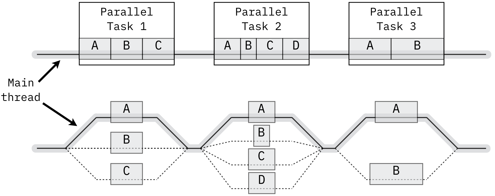
Figure 9.3.1: Illustration of sequential tasks (above) and the corresponding fork/join parallel implementation (below). Image source: Wikipedia (recreated)

Implementing the fork/join pattern in practice can be straightforward, particularly in the cases of embarrassingly parallel problems. The fork stage consists of setting up the arguments that each thread should receive. Code Listing 9.3, for example, shows how to break the loop from Code Listing 9.1 into 10 threads that each process 1/10^th of the array calculations (encapsulated in a multiply() function). The join stage would combine their results after calling pthread_join().

 1
 2
 3
 4
 5
 6
 7
 8
 9
10
11

/* Code Listing 9.3:
   The fork stage of a fork/join pattern
 */

for (i = 0; i < 10; i++) /* Assume we are creating 10 threads */
  {
    args[i].array = array;
    args[i].start = i * 100000000;
    assert (pthread_create (&threads[i], NULL,
                            multiply, &args[i]) != 0);
  }

The fork/join pattern is so common, particularly for loop parallelism, that many libraries provide simple mechanisms to automate the thread management for it when programming. Code Listing 9.4 shows the OpenMP version of parallelizing Code Listing 9.1. When the compiler encounters this pragma, it will inject code that handles the thread creation and cleanup with no additional work by the programmer. This pragma makes implementing the fork/join pattern trivial in this and many cases.

1
2
3
4
5
6
7

/* Code Listing 9.4:
   OpenMP works very well with embarrassingly parallel fork/join patterns
 */

#pragma omp parallel for
for (i = 0; i < 1000000000; i++)
  array[i] = i * i;

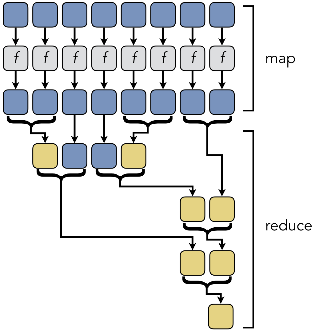
Figure 9.3.2: Map/reduce shares a common structure as fork/join

Map/reduce, shown in Figure 9.3.2, is another strategy that is closely related to fork/join. As in fork/join, a collection of input data is processed in parallel by multiple threads. The results are then merged and collected as the threads are joined until a single answer is reached. Although they are structurally identical, the type of work being done reflects a somewhat different philosophy. The idea behind the map stage is based on a technique in functional programming languages. A single function is mapped to all inputs to yield new results; these functions are self-contained and free of side effects, such as producing output. Several map stages can be chained together to compose larger functions. The map and reduce stages are also more independent than standard fork/join; mapping can be done without a reduction, and vice versa. Map/reduce is a popular feature in cluster systems, such as the Apache Hadoop system.

An implementation strategy common with task parallelism is the manager/worker pattern. In this scenario, independent tasks are distributed among several worker threads that communicate only with the single manager thread. The manager can monitor the distribution of the tasks to balance the workload evenly. To return to an earlier example, input event handlers are often implemented using the manager/worker pattern. In this case, the key press handler and the mouse event handler would each be implemented in separate workers; when either event occurs, the worker would inform the manager thread that would then process the data within the context of the program.

Code Listing 9.5 shows one way to structure a worker thread. The thread arguments contain a pointer to a piece of data to process (args->data) along with a lock (args->lock) and a condition variable (args->data_received). When the manager thread has a task to assign this particular thread, it would update the data pointer and send a signal with the condition variable. If each worker thread has its own data pointer, the manager can send data to a specific worker thread. On the other hand, if the data pointer is shared, this structure could still work; the main difference is that the thread would need to make a local copy of the data just before releasing the lock on line 17. Since condition variables also support broadcasting, the manager can send data to all of the worker threads with a single message. In addition, the thread arguments contain a boolean value args->running. The manager thread can stop all of the workers by setting this value to false and broadcasting on the condition variable (setting all args->data values to anything other than NULL).

 1
 2
 3
 4
 5
 6
 7
 8
 9
10
11
12
13
14
15
16
17
18
19
20
21
22

/* Code Listing 9.5:
   A simple worker with condition variables
 */

void *
worker (void * _args)
{
  struct args *args = (struct args *) _args;
  while (true)
    {
      /* Wait for the next available data */
      pthread_mutex_lock (args->lock);
      while (args->data == NULL)
        pthread_cond_wait (args->data_received, args->lock);
      if (! args->running)
        break;
      pthread_mutex_unlock (args->lock);
      /* Do something with the data here */
    }
  pthread_mutex_unlock (args->lock);
  pthread_exit (NULL);
}

9.3.3. Parallel Execution Patterns¶

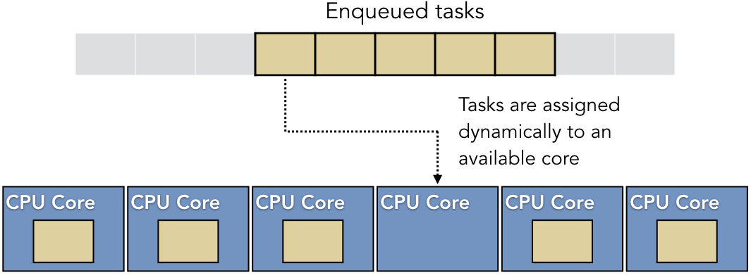
Figure 9.3.3: A thread pool retrieves tasks from the associated queue and returns completed results

Once the implementation strategy has been established, the software designer needs to make decisions about how the parallel software will run given the underlying hardware support available. One technique is to create a thread pool with an associated task queue. A thread pool is a fixed number of threads that are available for the program to use. As parallel tasks arrive, they are placed into a task queue. If a thread in the pool is available, it will remove a task from the queue and execute it. Figure 9.3.3 shows the logical structure of this approach.

At first glance, thread pools may look identical to the manager/worker implementation pattern described above. The difference is that the manager/worker pattern describes what is to be done, whereas the thread pool structure describes how it will be done. The master/worker pattern is in contrast to the fork/join pattern. Master/worker employs task parallelism, with different workers may be performing different tasks; fork/join employs data parallelism, with identical threads performing the same task on different data. A thread pool can be used for both approaches.

The main idea of a thread pool is to create all of the threads needed once at the beginning of the program, rather than when needed. Code Listing 9.3, for instance, did not use a thread pool to parallelize the loop. This could be contrasted with Code Listing 9.6, which assumes the presence of a thread pool. In this approach, the for-loop employs the producer-consumer enqueue() operation from Chapter 8 to place the starting values into the shared queue. The space and items semaphores help to ensure that the queue is modified safely. After enqueueing all of the data, the main thread waits at a barrier until the pool threads have reached the end of their calculations. The barrier prevents the main thread from moving past the fork/join structure until all of the pool threads have reached the same point.

 1
 2
 3
 4
 5
 6
 7
 8
 9
10
11
12

/* Code Listing 9.6:
   Using a thread pool to parallelize Code Listing 9.1
 */

/* Initialize barrier for this thread + 10 from the thread pool */
pthread_barrier_init (&barrier, NULL, 11);

/* Use the producer-consumer enqueue from Code Listing 8.15 */
for (i = 0; i < 10; i++)
  enqueue (queue, i * 100000000, space, items);

pthread_barrier_wait (barrier);

Code Listing 9.7 shows the structure of a thread in the thread pool. (For simplicity and focus on the thread pool, we are assuming all semaphores, the queue, the lock, and the barrier are globally accessible.) This thread starts by retrieving a piece of data from the shared queue, using the producer-consumer dequeue() operation. Note that, since there are multiple threads in the pool, this thread needs the dequeue() operation that employs a lock. This version synchronizes the pool threads’ access to the variables that maintain the queue structure. After retrieving the starting value (which was passed through the queue as a pointer), the thread performs the desired work and waits at the barrier (indicating completion to the main thread).

 1
 2
 3
 4
 5
 6
 7
 8
 9
10
11
12
13
14
15

/* Code Listing 9.7:
   The threads in the pool for parallelizing Code Listing 9.1
 */

void *
pool_thread (struct args *args)
{
  /* ... Declarations and other work omitted for brevity ... */
  /* Use the dequeue from 8.18, given multiple consumers */
  int starting = (int)dequeue (queue, space, items, lock);
  for (i = starting; i < starting + 100000000; i++)
    array[i] = i * i;
  pthread_barrier_wait (barrier);
  /* ... Additional work may happen later ... */
}

One way to characterize the difference between the thread pool approach in Code Listing 9.6 with the basic fork/join style of Code Listing 9.3 is to distinguish them as either a pull or a push model. Thread pools are typically implemented using a pull model, where the pool threads manage themselves, retrieving data from the queue at their availability and discretion. In contrast, the original approach used a push model, with the main thread controlling which thread accomplished which task.

The thread pool approach has several advantages. First, it minimizes the cost of creating new threads, as they are only created once when the program begins. Many naive multithreaded implementations fail to realize the benefits of parallelism because of the overhead cost of creating and managing the threads. Second, thread pools make the resource consumption more predictable. A simultaneous request to create a large number of threads could cause a spike in memory consumption that could cause a variety of problems in the system. Third, as just noted previously, thread pools allow the threads to be more self-managing based on local performance characteristics. If one thread is running on a core that is overloaded with other work, that thread can naturally commit less work to this task.

The self-management of thread pools can also be a disadvantage, as well. If there is no coordination between the threads and they are running on different processor cores, the cache performance may suffer, as data may need to be shuffled around frequently. Similarly, if there is no logging of which core takes which task or data set, responding to hardware failures might be difficult and data could be lost. Finally, the shared queue must be managed, which could induce performance delays in the synchronization that could otherwise be avoided.

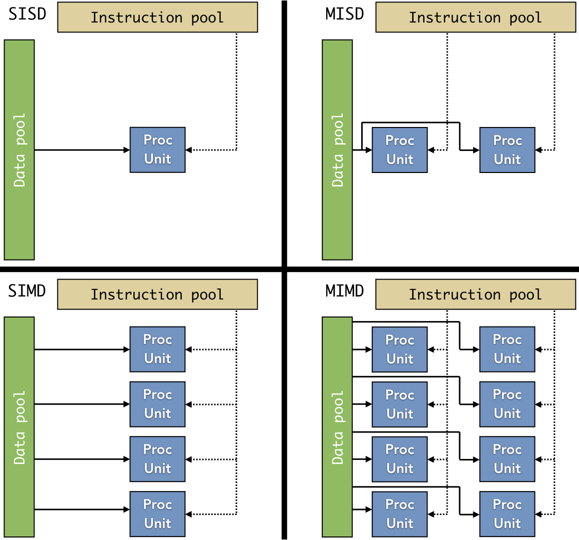
Figure 9.3.4: The four paradigms of Flynn’s taxonomy, showing how single/multiple instructions and single/multiple data are linked to processing units. Image source: Wikipedia (recreated)

Another factor that influences the execution of parallel systems is the capabilities of the hardware. Flynn’s taxonomy describes four paradigms of parallel hardware architectures in terms of the decompositions they support. Figure 9.3.4 illustrates the logical organization of each of the four paradigms. In each structure, a processing unit (“PU”) is provided with one or more parallel instructions (SI for “single instruction” and MI for “multiple instruction”) and performs the desired computation on a single input (SD) or multiple pieces of data (MD).

Traditional uniprocessing software adheres to the SISD model, as a single processor executes a single instruction on a single piece of data at a time; as such, SISD does not support parallel execution but is included in the taxonomy for completeness. Of the parallel models, SIMD is perhaps the most intuitive and the one with which most readers would be familiar. Modern CPUs provide SIMD support through various extensions to the ISA, such as the streaming SIMD extensions (SSE) or advanced vector extensions (AVX) for Intel processors, as well as the Neon or Helium instruction sets for ARM processors. Graphics processing units (GPUs) provide native support for SIMD operations, such as manipulating the rows of pixels in an image in parallel. Given this native support, GPUs are also widely used for applications that perform independent calculations in parallel. For instance, many scientific or security applications involve brute-force searches of a large set of data; GPU SIMD instructions can facilitate parallelizing the computations needed for these applications.

The MISD model is often confusing when first encountered, and many people do not immediately perceive its value as parallelism. One common use of MISD would be to provide fault tolerance in programs that require precision. The multiple instructions are all executed in parallel on the same input data; the results of the computations can then be evaluated to confirm that no errors occurred. Systolic array architectures, which are specialized systems for parallelizing adanced mathematical operations, can also be classified as MISD. For instance, specialized designs can optimize the parallel calculation of the multiplication and addition operations found in matrix multiplication. MISD hardware implementations are not common and are typically only found in custom hardware designs.

MIMD architectures allow the processors to work independently, performing different instructions on different pieces or sets of data at the same time. SPMD (single program, multiple data) is a common subset of MIMD in distributed computing; in SPMD, a single program with multiple instructions can be deployed independently to run in parallel. The key distinction between SPMD and SIMD is that SIMD instructions are synchronized. In a SIMD system, all processors are executing the same instruction at the same time according to the same clock cycle; SPMD architectures provide more autonomy, with each processor executing instructions independently of the rest of the system.

Large-scale parallel architectures, particularly MIMD, typically rely on a memory architecture that complicates their software development. In traditional SISD computing models (e.g., personal computers and laptops), all memory accesses are essentially equal; accessing a global variable near address 0x0804a000 takes the same amount of time as accessing a stack variable near 0xbfff8000. In large-scale MIMD systems, such as those used for high-performance computing, that claim is not necessarily true. These large-scale systems use non-uniform memory access (NUMA) designs. In NUMA, the memory hardware is distributed throughout the system. Some portions of memory are physically closer to a processing unit than others; consequently, accessing these closer portions of memory is faster than others.