2.2. Processes and Multiprogramming¶

2.2.1. Uniprogramming and Utilization¶

Early batch processing systems used a strategy known as uniprogramming. In uniprogramming, one program was started and run in full to completion; the next job would start immediately after the first one finished. The problem with this approach is that programs consisted of both CPU instructions and I/O operations. CPU instructions were very fast, as they consisted of electrical signals. I/O operations, however, were very slow. One example of an early I/O device was the drum memory, which was a large magnetic device that had to be mechanically turned for every data access. If a program required many I/O operations to be performed, that created a lot of wasted time where the CPU sat idle instead of executing instructions.

We can quantify this wasted time as the CPU utilization. In general terms, utilization can be defined mathematically as the actual usage of a resource divided by the potential usage. Utilization is reported as a unit-less ratio, typically a percentage. For instance, if a system is only used for half of the time that it could be, we would say that it experienced 50% utilization. In regard to CPU time, utilization is calculated as the following ratio:

Example 2.2.1

---

Consider the following timeline illustration for three sequential uniprogramming processes.

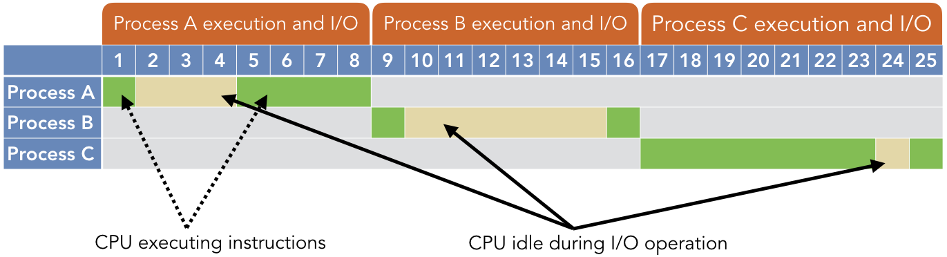
The green regions indicate times when the CPU is executing instructions in the program, while the yellow indicates that the times where the CPU is idle while waiting on an I/O operation to complete. The following table summarizes the time each process spends executing on the CPU or waiting for I/O:

Process	CPU time	I/O time
A B C	5 2 8	3 6 1
Total	15	10

In this scenario, the CPU was used for a total of 15 out of 25 possible seconds, so the system experienced 60% CPU utilization when running these three jobs:

$\large \mbox{CPU utilization} = \displaystyle\frac{5 + 2 + 8}{5 + 2 + 8 + 3 + 6 + 1} = \frac{15}{25} = 60\%$

As the preceding example illustrates, a significant amount of system resources can be wasted by waiting on I/O operations to complete. It should be noted that this problem still exists in modern systems. While modern I/O devices (such as solid-state drives) are significantly faster than memory drums, modern CPUs are also significantly faster than those in early machines. I/O bottlenecks tend to be among the most significant barriers to high-speed performance. Given that waiting on I/O operations to complete is slow and wasteful, system designers proposed a straightforward solution: switch to another process while an I/O operation is being performed.

2.2.2. Multiprogramming and Concurrency¶

In multiprogramming (also called multitasking), several processes are all loaded into memory and available to run. Whenever a process initiates an I/O operation, the kernel selects a different process to run on the CPU. This approach allows the kernel to keep the CPU active and performing work as much as possible, thereby reducing the amount of wasted time. By reducing this waste, multiprogramming allows all programs to finish sooner than they would otherwise.

Example 2.2.2

---

Consider the following timeline illustration for the same three processes from Example 2.2.1, but in a multiprogramming environment.

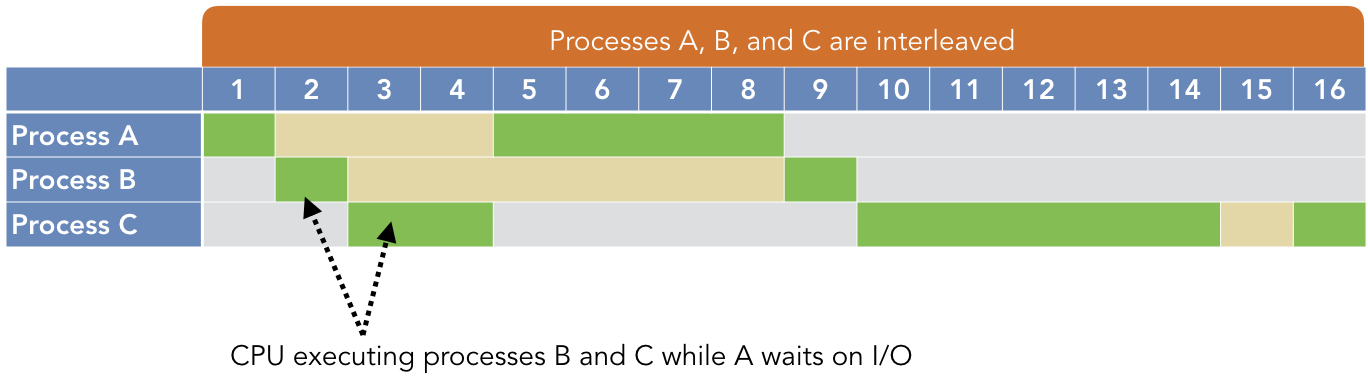
As before, the green regions indicate CPU execution and the yellow indicates I/O operations. However, note that processes B and C can run while A is waiting on its I/O operation. Similarly, A and C execute while B is waiting on I/O operations. As a result, the CPU is only completely idle while C’s I/O operation is performed at time 15, because A and B have already run to completion.

In our revised CPU utilization calculation, the numerator does not change because the total amount of CPU execution time has not changed. Only the denominator changes, to account for the reduced time wasted waiting on A’s and B’s I/O operations.

$\large \mbox{CPU utilization} = \displaystyle\frac{5 + 2 + 8}{5 + 2 + 8 + 1} = \frac{15}{16} = 93.75\%$

There are two forms of multiprogramming that have been implemented. The most common technique is preemptive multitasking, in which processes are given a maximum amount of time to run. This amount of time is called a quantum, typically measured in milliseconds. In preemptive multitasking, if a process issues an I/O request before its quantum has expired, the kernel will simply switch to another process early. However, if the quantum has expired (i.e., the time limit has been reached), the kernel will preempt the current process and switch to another. In contrast, with cooperative multitasking, a process can run for as long as it wants until it voluntarily relinquishes control of the CPU or initiates an I/O request.

Cooperative multitasking has a number of advantages, including its simplicity of design and implementation. Furthermore, if all processes are very interactive (meaning they perform many I/O operations), it can have low overhead costs. However, cooperative multitasking is vulnerable to rogue processes that dominate the CPU time. For instance, if a process goes into an infinite loop that does not perform any I/O operation, it will never surrender control of the CPU and all other processes are blocked from running. As a result, modern systems favor preemptive multitasking.

By providing a mechanism for increasing CPU utilization, multiprogramming creates the foundation for concurrent execution of software. Concurrency, in this context, can be thought of as the appearance of simultaneous program execution. That is, concurrency through multiprogramming is what makes it possible to use a web browser while listening to music with an MP3 player at the same time. Throughout most of the history of computing, these applications were not actually executing code at the same time; rather, the kernel was just switching back and forth between them so quickly that users could not notice.

A simple way to illustrate multiprogramming in modern software is with the sleep() function. This function’s only argument is the number of seconds to pause the current process. During this time, the system will switch to other processes that need to run. In other words, calling sleep() can be interpreted as a form of cooperative multitasking.

C library functions - <unistd.h>

---

unsigned sleep(unsigned seconds);

Suspend the current process for a number of seconds.

Code Listing 2.2 shows an example of using sleep() to introduce repeated pauses in a process’s execution. This code will print “Hello!” 10 times, pausing for one second between each print. By running this code along with other programs (such as a media player or web browser), you can clearly observe that your computer is still operating during these 10 seconds. In fact, this can be made even clearer by running the same program in multiple windows; each instance will take turns printing the message and sleeping along with the others.

1
2
3
4
5
6
7
8
9

/* Code Listing 2.2:
   Repeatedly pausing the current function to illustrate multiprogramming
 */

for (int i = 0; i < 10; i++)
  {
    printf ("Hello!\n");
    sleep (1);
  }

2.2.3. Context Switches and Overhead Costs¶

Context switches form the basis of multiprogramming. A context switch is the change from one process’s virtual memory image to another. In a context switch, the kernel portion of virtual memory does not change. However, the user-mode code, data, heap, and stack segments that the CPU uses are changed. It’s important to note that both the old and new processes still reside in physical memory – the hardware memory component – simultaneously. The difference is that the kernel has changed which portion of physical memory is actively being used for the virtual memory image.

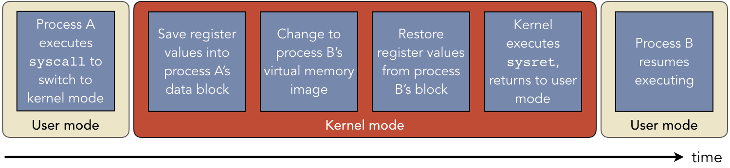
Figure 2.2.6: Timeline showing the major events in a context switch from process A to process B

Although context switches are critical for multiprogramming, they also introduce complexity and overhead costs in terms of wasted time. First, when the kernel determines that it needs to perform a context switch, it must decide which process it will now make active; this choice is performed by a scheduling routine that takes time to run. Second, context switches introduce delays related to the memory hierarchy. In early cache systems, a context switch required all cache data to be invalidated. As such, all cache data for the old process had to be flushed and replaced with the new process’s data. Newer systems allow different parts of the cache to be associated with different processes; however, this reduces the total amount of data that the cache can store, increasing the number of cache misses.

Because context switches introduce overhead costs, kernel designers strive to reduce their impact on performance. One way to do this is to increase the quantum given to each process, thereby letting it run longer before forcing a context switch. In fact, this is the main idea behind cooperative multitasking, which can be viewed as providing an infinite quantum to each process. The risk is that increasing the time quantum too much allows some processes to dominate the CPU time, effectively monopolizing the system resources. Empirical research on this trade-off has led to a common practice of 4 - 8 ms per quantum in modern systems.