9.6. Reliable Data Storage and Location¶

9.6.1. Google File System¶

As an example of how replication provides reliable service for data storage, consider the Google File System (GFS). Figure 9.6.1 shows the structure of the main components of GFS. In GFS, the assumption is that files are large (e.g., each file might be multiple terabytes in size), so they are broken up into chunks. The individual chunks with the file contents are stored on chunkservers. Each of these chunkservers contains its own traditional local file system; for example, assuming the machines are running Linux, then the chunks would be stored as local files within that chunkserver’s ext4 file system. In addition, a GFS master maintains a non-authoritative table that maps files to their locations.

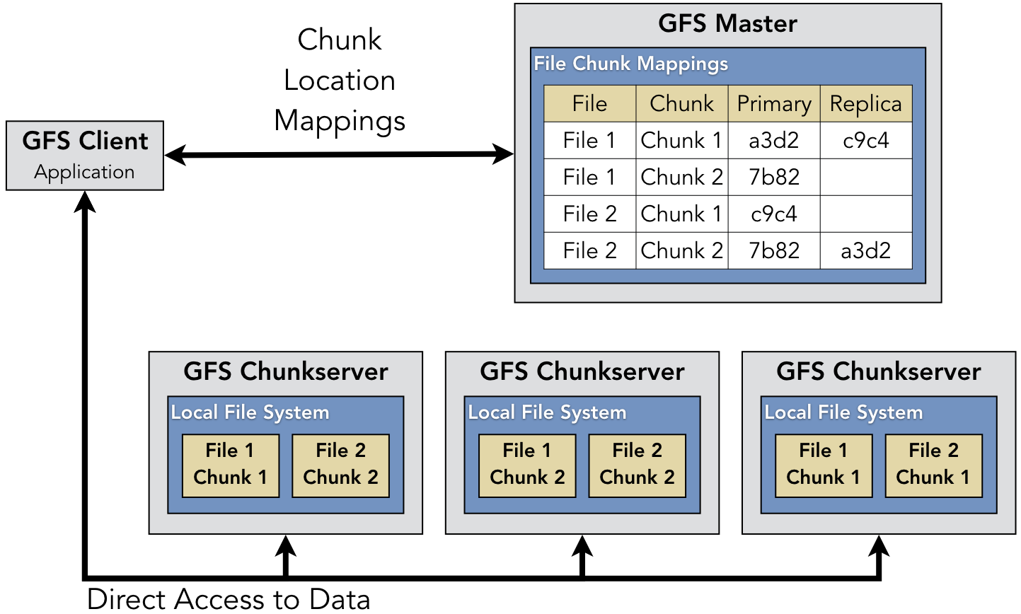
Figure 9.6.1: The structure of the Google File System (GFS)

For each given chunk, there is a designated primary chunkserver along with multiple replicas. The primary and replicas all store identical copies of the chunks, but the primary is designated as having a lease on the file and has exclusive access to modify it if needed. For instance, in Figure 9.6.1, the first chunk of File 1 can be retrieved from either node a3d2 (the left-most chunkserver) or node c9c4 (the right-most). Ultimately, each chunkserver has full control over the chunks that it stores, and this information might differ from the records in the GFS master. To keep the GFS master’s records updated, the GFS master sends out periodic HeartBeat messages to the chunkservers to determine their current status and provide additional instructions.

9.6.2. Distributed Hash Tables¶

GFS was designed to create a distributed file system for a single organization. Consequently, Google could build in some assumptions into the design about the locations of nodes. When the GFS master in Figure 9.6.1 informed the client that node a3d2 was the assigned primary for chunk 1 of file 1, the client knew which machine to contact, because the clients maintain information about the IP addresses of nodes in the system. In other distributed file systems—particularly those designed to be openly accessible—clients do not have this information.

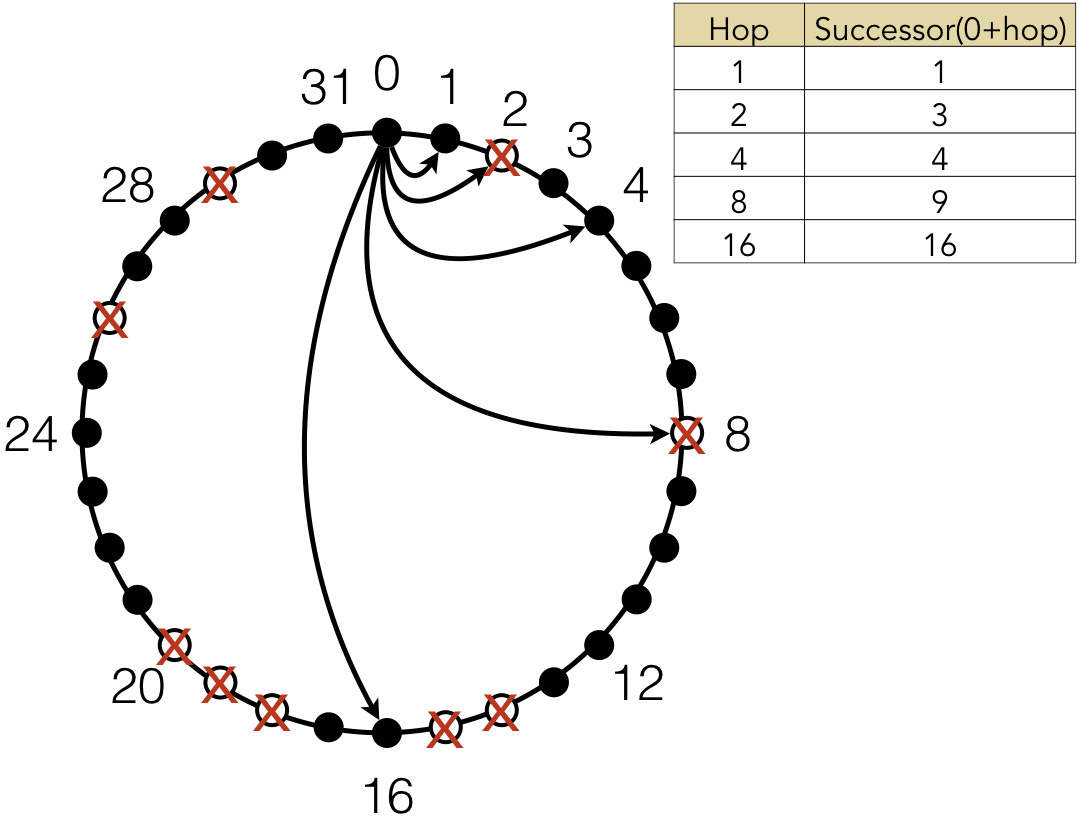
Figure 9.6.2: A Chord ring with up to 32 nodes. Black nodes are live (available); nodes with a red X are considered failed (absent or unavailable)

Instead of relying on the clients to have information about node locations, systems can create a distributed hash table (DHT) that maps objects to machines that host them. Chord was an early [1] and influential DHT. In Chord, all nodes were assigned unique identifiers and arranged in a logical ring structure. Figure 9.6.2 shows the logical structure of a simplified Chord ring with support for 32 nodes. (Chord node identifiers are created by calculating the hash of the machine’s IP address; for a 256-bit hash value, the ring would have up to $2^{256}$ nodes.) Most of the nodes are live, meaning those machines are running and connected to the system; nodes marked with an X (e.g., 2, 8, and 14) are not connected.

Figure 9.6.2 also shows a key data structure to define the nature of the Chord ring: the finger table. Every node contains a finger table, which contains information about other Chord ring indexes. Each entry in the finger table is based on the current node’s identifier plus a power of 2. The finger table shown here would be the table for node 0. Node 0 would contain information about the indexes 1, 2, 4, 8, and 16 (i.e., $0+2^0$, $0+2^1$, $0+2^2$, $0+2^3$, and $0+2^4$). Similarly, node 1 would contain information about 2, 3, 5, 9, and 17 ($1+2^0$, $1+2^1$, $1+2^2$, $1+2^3$, and $1+2^4$). However, given that some nodes are missing (such as 2 and 8), Chord nodes keep track of the successor of the target index, which is the closest value greater than or equal to the index. Since 1, 4, and 16 are present, these nodes are their own successors. Since 2 and 8 are missing, 3 is the successor of 2 and 9 is the successor of 8. Within the finger table, the Chord nodes keep track of information about that successor, including its IP address.

The logical ring structure of Chord makes it possible for items to be located very efficiently, even though nodes in the system have very little information about the structure. Assume that a user is running a client on node 6. This user tries to open the file "chord/data/foo". As with the node identifiers, objects are mapped to keys using hashes, so the user would calculate the hash of the file name. If "chord/data/foo" hashes to the value 19, then the successor of 19 is deemed the location of that object.

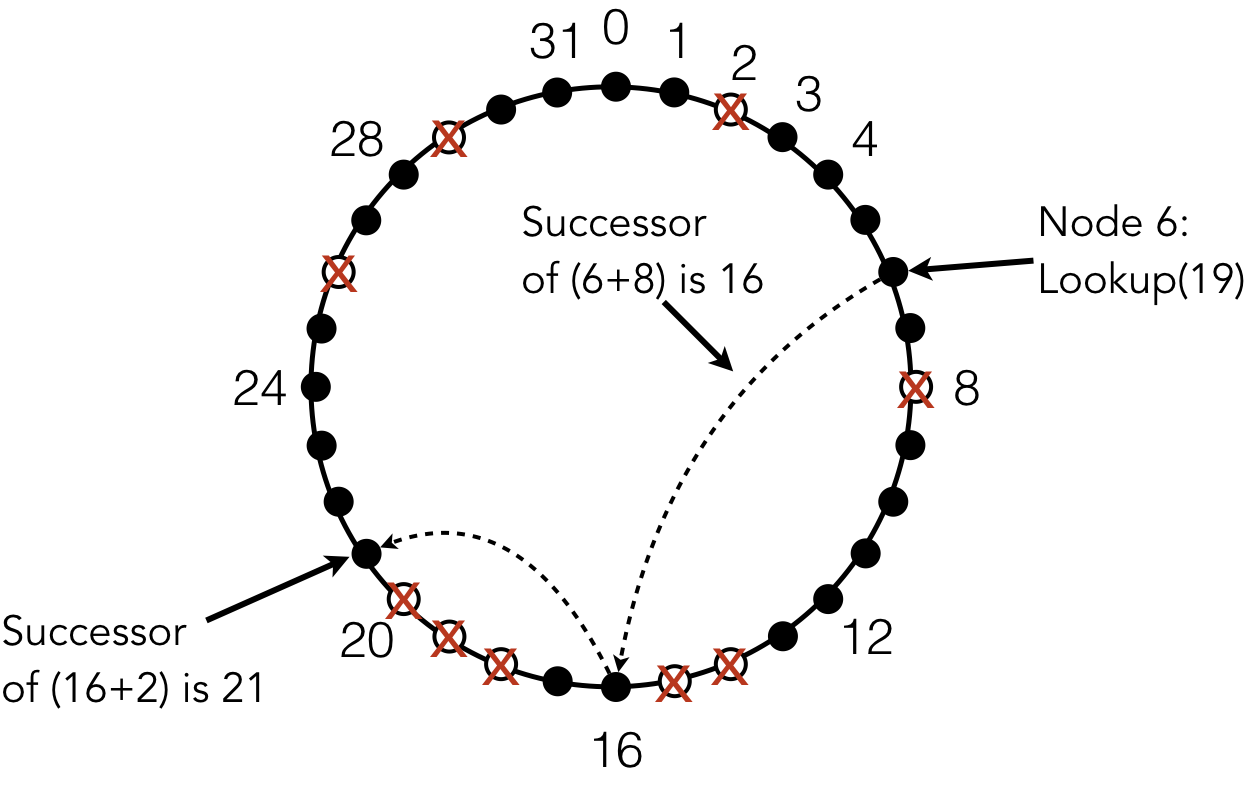
Figure 9.6.3: Routing a Chord lookup message for key 19 from node 6 to node 21

Figure 9.6.3 shows the routing of the request message through the Chord ring. Node 6 would have entries for the successors of 14 ($6+2^3$) and 22 ($6+2^4$). Since 22 is greater than the target key 19, node 16 would try to contact the successor of 14. Since node 14 is absent from the ring, node 6 would actually contact node 16. Note that node 6 determines this itself, because this information is stored in its own finger table. When node 16 receives the request for key 19, it would find the successor of 18, which is $16+2^1$. Since nodes 18, 19, and 20 are all missing, node 21 is the successor of 18, so this node is the location of the requested file.

The routing structure of Chord is deceptively powerful. Although it seems complicated, the structure is straightforward to implement in code. Code Listing 9.10 illustrates the algorithm for this lookup procedure. The logic of the algorithm is to start with the last entry of the finger table (assuming 64 entries because of 64-bit integer types; supporting a 256-bit identifier would require larger integer types) and work backwards to find the first entry that precedes the key.

 1
 2
 3
 4
 5
 6
 7
 8
 9
10
11
12
13
14
15
16
17
18
19
20

/* Code Listing 9.10:
   Algorithm for finding the next node in a Chord finger table
 */

#define NUM_ENTRIES 63 /* assume all keys are 64 bits */
uint64_t
lookup (uint64_t key)
{
  for (int index = NUM_ENTRIES; index > 0; index--)
    {
      if (node_id < finger_table[index])
        {
          if (key >= finger_table [index] || key < node_id)
            return finger_table [index];
        }
      else if (key >= finger_table [index] && key < node_id)
        return finger_table [index];
    }
  return node_id; /* default response is current node */
}

The logic in Code Listing 9.10 is complicated by the modular arithmetic imposed by the Chord ring structure. Essentially, the algorithm starts by looking at node_id + 2^max and incrementally decreases the exponent. Each time, the algorithm checks that the key would occur after the jumped node but before the current node. For instance, considering the lookup in Figure 9.6.2, the algorithm would look at $6+^2$4, to check if the key lies after 22 but before 6; if so, the algorithm would return 22 as the next node to jump to, otherwise it would look at $6+2^3$. If we consider a similar query, though, starting from node 18, the algorithm would first look at $18+2^4$, but this value must be mapped to the ring by applying mod 32. As such, the algorithm would need to check if the key comes after node 2 and before node 18. With modular arithmetic, determining whether a key value is between two nodes on the ring can be tricky to get the logic correct.

The benefit of the Chord structure is that it places a very efficient upper-bound of Θ(log n) on the number of messages to find an object in the system. To put that into practical figures, given a system with 1,000,000 nodes storing data, any item could be found by forwarding the request at most 20 times. If the number of nodes doubles, the maximum number of request messages would only increase by one. Consequently, the network overhead with Chord is very light.

To improve the system performance further, Chord also employs replication through caching. Whenever a node is involved in looking up an object’s location, that node receives a copy of the object, as well. Returning to Figure 9.6.2, since node 16 was used as a step toward locating key 19 at node 21, node 16 also gets a copy. At that point, any request for the file "chord/data/foo" that goes through either node 6 or 16 will get a faster response. Since these nodes have a local replica of the file, there is no need to forward the request. Because of this caching technique and other forms of replication, Chord provides efficient times to find objects and high levels of availability (even when nodes fail).