PA 3: Sorting

Introduction - What is the World's Best Sorting Algorithm?

Old: Fix for VS Code Tests

Updated 4/7: As of 4/7/2025, it appears that the issue has been fixed with an update to the "Test Runner for Java" extension. If you previously applied the fix below, and are now having issues, please update all extensions and restart VS Code.

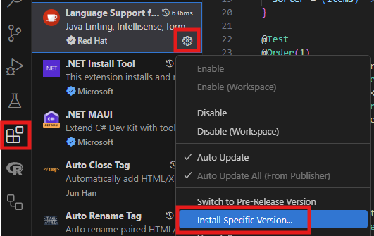
If you are using VS Code, as of 4/2/2025, version 1.41.1 of the "Language Support for Java(TM) by Red Hat" extension broke discovery of tests for Java. If your testing pane is empty or the "run test" buttons are missing, please install a previous version of the extension:

1. Open the extensions pane on the left (Ctrl+Shift+X or Cmd+Shift+X).
2. Locate the "Language Support for Java(TM) by Red Hat" extension.

3. Click the gear icon next to it and select "Install Specific Version...".

   

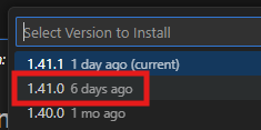
4. In the popup at the top, select version "1.41.0" (not "1.41.1").

   

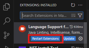
5. Once installed, either "restart extensions" or restart VS Code.

   

There is no single best sorting algorithm. Quicksort is the fastest known comparison-based sorting algorithm when applied to large, unordered, sequences. It also has the advantage of being an in-place (or nearly in-place) sort. Unfortunately, quicksort has some weaknesses: it's worst-case performance is \(\Theta(n^2)\), and it is not stable. Merge sort shares neither of these disadvantages: it is stable and it requires \(\Theta(n \log n)\) steps in the worst case. Unfortunately, merge sort requires \(\Theta(n)\) additional space and it runs more slowly than quick sort on most inputs.

What we really want is a sorting algorithm that is as fast as quicksort, stable, in-place, with \(\Theta(n \log n)\) worst-case performance. Sadly, no such algorithm has yet been discovered. In practice, most code libraries follow one of two paths: either they provide a modified version of quicksort that is able to avoid worst-case behavior on typical inputs, or they provide a modified version of merge sort that is able to close some of the performance gap through careful optimizations¹.

The objective of this assignment is to write modified versions of merge and quicksort that exhibit better performance than the standard versions described in our textbook. You will implement three improvements (two for merge sort and one for quicksort) that should improve some aspect of the algorithm's performance without requiring a great deal of additional code. You will also experimentally evaluate the impact of your improvements.

Starter Code

The following zip file contains starter code, including the sort implementations provided by our textbook.

sorting.zip

This zip file has the following contents:

• Sorting algorithms:
  • BasicSorts.java - Includes selection sort and insertion sort. (UNFINISHED. See Part 2 below.)
  • MergeSort.java - Includes merge sort.
  • QuickSort.java - Includes quicksort.
  • MergeSortImproved.java (UNFINISHED. See Parts 1 & 2 below.)
  • IntrospectiveSort.java (UNFINISHED. See Part 3 below.)
• An example of how to analyze the performance of sorting algorithms:
  • AnalyzeSorts.java - A simple driver that demonstrates how to count operations for the basic provided sorts
• And the ArrayWrapper class:
  • The ArrayWrapper.java class provides a wrapper around a standard Java array, allowing for more controlled manipulation and analysis of sorting algorithms.
  • Instead of directly sorting a Java array, all operations must be performed on an ArrayWrapper object. This class internally maintains an array and provides methods such as get, set, and swap to access and modify its values.
  • Additionally, ArrayWrapper includes the getTotalOperations method, which tracks the total number of operations performed since the last reset. The primary motivation for using ArrayWrapper instead of a raw Java array is to facilitate performance analysis.

ArrayWrapper Example

You can use the ArrayWrapper like so:

ArrayWrapper<Integer> myArray = new ArrayWrapper<>(10); // Create an array of size 10

myArray.set(0, 5); // Set the first element (index 0) to 5
myArray.set(1, 3); // Set the second element (index 1) to 3

myArray.swap(0, 1); // Swap the first and second elements

for (int i = 0; i < myArray.length(); i++) { // NOTE: .length() is a METHOD!
    int value = myArray.get(i);
    System.out.println(value);
}

The ArrayWrapper class allows you to count operations performed by a sorting algorithm. You are not allowed to use regular Java arrays for this assignment. You must use the provided ArrayWrapper class.

Additionally, you may not call resetTotalOperations in your sorting algorithms. This method is only for use in the AnalyzeSorts class when measuring the number of operations.

Measuring Time vs. Counting Operations

When comparing sorting algorithms, one approach is to implement them and measure their execution times. However, fair comparisons can be challenging since the runtime of many sorting algorithms depends on the specific characteristics of the input values, the performance of the computer, and other real-world factors.

By using the ArrayWrapper class, we can analyze sorting algorithms more effectively by measuring the cost in terms of the number of operations performed on the underlying array, providing a more controlled and insightful comparison.

Part 1 - Improved Merges

In this part, you need to complete the mergeSortHalfSpace methods in MergeSortImproved.java.

Recursive Helper Method

Because the mergeSortHalfSpace method is recursive, you will need to implement a recursive helper method that takes additional parameters to specify the range of the array to sort. This helper method should be kept private.

See the provided mergeSort method in MergeSort.java for an example!

The merge algorithm described in our textbook consists of the following two stages:

1. Merge the values from the two pre-sorted halves into a temporary array.
2. Copy the values from the temporary array back into the original array.

If \(n\) is the combined size of the two sub-arrays being merged, this algorithm requires a temporary array of size \(n\), and requires \(n\) assignment operations in stage 2. The following alternative approach cuts both of those values from \(n\) to around \(n/2\):

1. Copy the values from the first pre-sorted half to a temporary array.
2. Merge the values from the temporary array and the second
   pre-sorted half into the original array.

Some ASCII graphics will help illustrate this process. Suppose these are the two sorted sub-arrays that need to be merged:

Original sorted sub-arrays:

      ________________________________________
  ...| 1 | 3 | 5 | 7 | 9 | 2 | 4 | 6 | 8 | 10 |...
      ----------------------------------------
 start-^           mid-^               end-^

Instantiate a temporary array large enough for the first sorted sub-array:

      ___________________
     |   |   |   |   |   |
      -------------------
     0-^

      ________________________________________
  ...| 1 | 3 | 5 | 7 | 9 | 2 | 4 | 6 | 8 | 10 |...
      ----------------------------------------
 start-^           mid-^               end-^

Copy the sorted first half into the temporary array:

         ___________________
        | 1 | 3 | 5 | 7 | 9 |
         -------------------

         ________________________________________
     ...|   |   |   |   |   | 2 | 4 | 6 | 8 | 10 |...
         ----------------------------------------

Initialize tmpIndex to be the index of the first position (0) in the temporary array, rightIndex to be the index of the first position of the sorted right half, and mergeIndex to be the next available position for merging:

          ___________________
         | 1 | 3 | 5 | 7 | 9 |
          -------------------
  tmpIndex-^
         ________________________________________
      ...|   |   |   |   |   | 2 | 4 | 6 | 8 | 10 |...
         ----------------------------------------
mergeIndex-^        rightIndex-^

Since temp[tmpIndex] < items[rightIndex], temp[tmpIndex] is copied to items[mergeIndex]. tmpIndex and mergeIndex are incremented.

       ___________________
      | 1 | 3 | 5 | 7 | 9 |
       -------------------
   tmpIndex-^
       ________________________________________
   ...| 1 |   |   |   |   | 2 | 4 | 6 | 8 | 10 |...
       ----------------------------------------
 mergeIndex-^    rightIndex-^

Since items[rightIndex] < temp[tmpIndex], items[rightIndex] is copied to items[mergeIndex]. rightIndex and mergeIndex are incremented.

       ___________________
      | 1 | 3 | 5 | 7 | 9 |
       -------------------
   tmpIndex-^
       ________________________________________
   ...| 1 | 2 |   |   |   | 2 | 4 | 6 | 8 | 10 |...
       ----------------------------------------
     mergeIndex-^    rightIndex-^

Continue Merging until complete:

       ___________________
      | 1 | 3 | 5 | 7 | 9 |
       -------------------
       ________________________________________
   ...| 1 | 2 | 3 | 4 | 5 | 6 | 7 | 8 | 9 | 10 |...
       ----------------------------------------

We recommend writing tests to verify that your implementation is correct and sorting the array as expected. The AnalyzeSorts class provides a few protected methods that can help generate test cases for you.

We have also given you the example code for the regular mergeSort -- reference it when writing your mergeSortHalfSpace method.

Part 2 - Switching Strategies

In this part, you need to complete:

1. insertionSubsort method in BasicSorts.java.

2. The mergeSortAdaptive methods in MergeSortImproved.java.

   • Again, one of these methods will be a recursive helper method.
   • Updated 3/23: mergeSortAdaptive should use the mergeHalfSpace method from Part 1 to merge two sub-arrays.

The next improvement is based on the observation that merge sort is actually slower than simple \(\Theta(n^2)\) sorts for small input sizes. This may seem surprising given that merge sort is an \(\Theta(n \log n)\) sorting algorithm. However, it is important to keep in mind that asymptotic analysis is only concerned with rates of growth. A \(\Theta(n \log n)\) algorithm will always be faster than a \(\Theta(n^2)\) algorithm eventually, but that doesn't mean the \(\Theta(n^2)\) algorithm can't be faster for small inputs. The following figure was created by comparing merge sort and insertion sort on small randomly ordered arrays from size 2 to size 100:

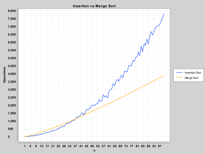
As you can see, insertion sort is faster until around \(n = 37\). At that point, merge sort becomes faster and it remains faster for all larger inputs. One of the largest costs of merge sort is the overhead needed to create a temp array at the start of the process and the need to copy values to this temp array for every merge.

A a reminder, the following pseudocode describes the overall logic of the merge sort Algorithm:

merge_sort(sub-array)
    If sub-array is has more than one entry:
        Recursively merge_sort the left half
        Recursively merge_sort the right half
        Merge the two sorted halves.

This logic recursively splits the original array into smaller and smaller sub-arrays until the recursion bottoms out at sub-arrays of size one. This means that every time a large array is sorted, there are many recursive calls to merge sort that have small input sizes. In light of the figure above, that approach doesn't make much sense: merge sort is not a competitive sorting algorithm on small inputs. It would make more sense to recursively break the input into smaller and smaller pieces until some threshold is reached, and then switch strategies to a sorting algorithm that is more efficient on those small inputs.

The following pseudocode describes this alternate approach:

merge_sort(sub-array)
    If sub-array has fewer than MERGE_SORT_THRESHOLD entries:
        Sort the sub-array with insertion sort.
    Otherwise:
        Recursively merge_sort the left half
        Recursively merge_sort the right half
        Merge the two sorted halves.

Choosing an appropriate value for MERGE_SORT_THRESHOLD requires some experimentation. One of the requirements of this assignment is that you select an appropriate threshold value and provide data to justify your choice.

Common Misconception

Simply selecting the crossover point (n=37) based on the figure above is not a reasonable strategy. The point where the two lines cross represents the input size where the two sorts are equally fast. Switching strategies at that input size will result in no speedup at all.

In fact, do not use the figure above to select a threshold value. Nor should you make your own version of the figure above. The figure is provided to illustrate a point, not to be used as a guide for selecting a threshold value.

The only way to determine an appropriate choice for MERGE_SORT_THRESHOLD is to systematically experiment with different threshold values until you find the one that leads to the best overall sorting performance.

You will need to create a method in AnalyzeSorts.java that tests how well mergeSortAdaptive performs for different values of MERGE_SORT_THRESHOLD. Your goal is to figure out which threshold value leads to the lowest number of operations for mergeSortAdaptive. You should repeat your experiment for a few different values of n to ensure you have picked a threshold that works well across a range of input sizes.

You should thoroughly test your implementation to ensure that it is working correctly before running any experiments. You will then report on your findings and make a graph for Part 4.

Hint: Expected Graph

You should end up with a graph that looks something like this:

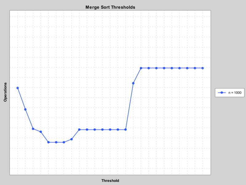
You can see how the graph dips down then increases after some point. The lowest point in that dip will mark the ideal threshold value for MERGE_SORT_THRESHOLD.

You should repeat your experiment with multiple values of n so that you can pick a threshold that works for multiple input sizes. You can plot the results for each value of n on the same graph to see how they compare.

Do not just try to replicate the example above; you should be more thorough in your analysis. Try a wide range of threshold values and multiple input sizes (e.g., n = 1000, 5000, 10000, ...).

Finally, note that we have provided an implementation of insertion sort that works on a full array, but you will need a version that works on a sub-array for this part of the assignment.

Part 3 - Introspective Sort

In this part, you will complete:

1. The introspectiveSort method in IntrospectiveSort.java.

   • This will also require a recursive helper method.
   • Updated 3/14: Do not rewrite the partition algorithm -- you should be able to call certain methods from QuickSort.java.

2. The mergeSubsortAdaptive method in MergeSortImproved.java.

   • You need this so that you can call it from introspectiveSort.

As mentioned above, quicksort is usually very fast. There are relatively few pathological inputs that result in \(\Theta(n^2)\) performance. The idea behind introspective sort is to perform a standard quick sort until there is evidence that the current input is pathological. If it looks like the current input will cause \(\Theta(n^2)\) performance, the algorithm switches strategies to a sorting algorithm with guaranteed \(O(n \log n)\) performance. Typically, heap sort is used as the alternative, since it is in-place and takes \(\Theta(n \log n)\) time in the worst case. Since we haven't yet studied heap sort, your version of introspective sort should use the adaptive merge sort from Part 2 as the alternate sorting algorithm. The resulting algorithm is almost as fast as quick sort for most inputs, but has a worst case performance of \(\Theta(n \log n)\).

It is possible to detect pathological inputs by tracking the recursion depth of the quicksort algorithm. When quicksort is working well, the partition operation typically moves the pivot item somewhere near the center of the current sub-sequence. When this is the case, the maximum recursion depth will be \(\Theta(\log n)\).

Therefore, introspective sort should switch strategies when the recursion depth exceeds \(2 \lfloor \log_2 n\rfloor\).

Updated 3/23: There are a number of possible variations on the basic Introsort algorithm. Your implementation should conform to the following pseudocode:

introspective_sort(array)
    introspective_sort(array, 2 ⌊log₂(array.length)⌋)

introspective_sort(sub-array, depth-limit)
    If depth-limit is 0
        merge_sort(sub-array)
    Otherwise
        If sub-array has 0 or 1 entries
            return
        Otherwise
            pivot ← partition(sub-array)
            introspective_sort(sub-array[0 to pivot - 1],
                               depth-limit - 1) 
            introspective_sort(sub-array[pivot + 1 to end],
                               depth-limit - 1)

Note that the provided version of merge sort sorts a full array. Introspective sort needs to be able to call a version of merge sort that can sort a portion of a provided array. The MergeSortImproved class provides a declaration for such a method.

Note that the provided version of merge sort sorts a full array. Introspective sort needs to be able to call a version of merge sort that can sort a portion of a provided array. The MergeSortImproved class provides a declaration for such a method.

Part 4 - Experimental Analysis

So far in this course we have focused on asymptotic analysis. This usually gives us the information we want. When deciding between two algorithms we generally prefer the one with better asymptotic performance.

Our goals for this project are somewhat different. The focus now is on fine-tuning existing algorithms to improve their performance. This is a situation where we really care about the constant factors. (We would be very happy if we could write a version of merge sort that is twice as fast, even if the asymptotic worst-case performance were still \(\Theta(n \log n)\).)

In order to help you evaluate your sorting improvements, we have given you an example in AnalyzeSorts.java that demonstrates how to count the number of operations performed by the four basic sorting algorithms and produce the results in a comma-separated value (CSV) format. You can use this example as a starting point for your own experiments.

Graphing the Results

The example in AnalyzeSorts.java produces values like the following:

n,insertion,selection,merge,quick
1,0,0,1,9
2,5,6,12,11
3,6,14,29,23
4,19,24,46,30
5,29,36,65,48
6,35,50,90,51
7,44,66,113,66
8,61,84,138,76
...

This is essentially a table of values! The first row is the header row, and the subsequent rows are the data. You can see how the first column represents n, followed by the number of operations for each sorting algorithm at that input size.

CSV data can be easily imported into a spreadsheet program like Microsoft Excel, Google Sheets, or even Desmos. You can then use the spreadsheet program to create graphs that compare the performance of the different sorting algorithms.

For example, you can copy the CSV data (including headers), paste it into Google Sheets, and then click "Split data into columns" to turn it into a table. In Excel, you can use the "Paste > Use Text Import Wizard" to do the same thing.

Afterwards, you will need to plot your results into an interpretable chart/graph. You should be able to figure out how to do this for your respective spreadsheet program.

• Google Sheets
• Excel
• Desmos

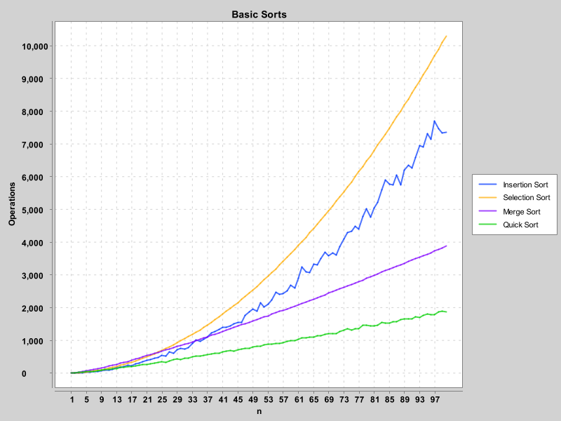
Example Graph

Here is an example of what a graph might look like:

Recommendations

Updated 3/14:

When creating your graphs, you should consider the following:

• We recommend creating "XY scatterplots", where the X axis represents n, and the Y axis represents the number of operations.
  • See above for an example!
• You should adjust the Y-axis range to easily see the entirety of the data.
  • If you use a 1-to-1 XY scale, the graph will be too tall and skinny to be useful.
  • As in the example above, you may want to plot operations by the thousands, so that the graph is more readable.
• If you are comparing two algorithms, they should be plotted on the same graph (otherwise, it is difficult to compare them).
  • Make sure to use different colors or symbols to differentiate between the two algorithms.
  • You should also include a legend to indicate which color/symbol corresponds to which algorithm.
• If recommended, you may elect to create two graphs for some parts.
  • Such as one graph for random inputs and another for ordered inputs.
  • Within each graph, you should still plot all algorithms together.
• Make sure to label your axes and include a title for your graph.

You will be graded based on how clearly labeled and interpretable your graph is and how well it supports your conclusions.

Your Report

For this part of the project you will prepare a short report that quantifies the performance improvements you were able to achieve.

The report will be in the form of a quiz on Gradescope. You will submit each figure/graph followed by a short paragraph describing the results illustrated in the figure.

You will need the following:

• Figure 1 - Improved Merges. This figure should compare the performance of mergeSortHalfSpace to the original merge sort implementation as well as quicksort. Results should be shown for both random and ordered inputs. To avoid clutter, it may be helpful to plot the results for random inputs and ordered inputs separately.
• Figure 2 - Threshold Selection. This figure should show the graphed data you used to select an appropriate threshold for switching strategies in mergeSortAdaptive.
• Figure 3 - Switching Strategies. This figure should compare your tuned mergeSortAdaptive to the previous two merge sort implementations as well as quicksort. Results should be shown for both random and ordered inputs.
• Figure 4 - Introspective Sort (Random Inputs). This figure should compare introspective sort to quicksort for randomly generated inputs.
• Figure 5 - Introspective Sort (Pathological Inputs). This figure should compare introspective sort to quicksort for worst-case quicksort inputs.

Each figure must have clearly labeled axes, a caption, and appropriate legends. Again, make sure your axes are scaled appropriately to show all the data clearly in a reasonable amount of space. We should not see any extremely tall or wide graphs.

The description must provide enough information for the reader to understand the point of the experiment and how the data supports the conclusion. You should describe things like what you expected, how the graph shows that, and your final conclusion. If there are any unexpected results, you should definitely mention them in your paragraphs.

Here are some examples of how paragraphs would be graded:

Submission

Submit the following four files to Gradescope:

• BasicSorts.java
• MergeSortImproved.java
• IntrospectiveSort.java
• AnalyzeSorts.java

Updated 3/14: You will only receive points for a sorting algorithm after passing all its respective tests, so make sure to test and debug your code thoroughly.

There will be a point deduction for excessive Gradescope submissions, but we recommend submitting to Gradescope immediately after finishing each part. Then go back and test/debug your code, and spend 2-3 more submissions to fix any errors. This will help you catch any issues early and ensure you are on the right track.

Updated 3/28: Make sure you include all four files every time you submit! Even if you have only completed one part, you should still include all four files.

Don't forget to submit your experimental results report to a separate Gradescope assignment!

Grading

Gradescope Tests for Improved Merge	20 points
Gradescope Tests for Switching Strategies	20 points
Gradescope Tests for Introspective Sort	20 points
Experimental Results Report	25 points
Instructor Style Points	10 points
Gradescope Style Checks	5 points
Excessive Submission Deduction	You have 20 free submissions, with -1 for each additional submission beyond 20.

The grading of your experimental evaluation will be based on the quality of the figures as well as the clarity of your writing.

---

1. The second approach has recently become popular. Both Python (starting in version 2.3) and Java (starting in version 7) use Timsort as their default sorting algorithm. Timsort is a modified version of merge sort that includes several enhancements: it uses a more space-efficient merge operation, it takes advantage of partially sorted arrays by finding and merging existing sorted regions, and it uses a non-recursive binary insertion sort to handle short unsorted regions. ↩