CS 354 Autonomous Robotics
Fall 2020
Introduction
The purpose of this assignment is to introduce the RRT and RRT* probabilistic planning algorithms and to investigate their performance characteristics in terms of runtime and path quality.
Resources
- Lecture Slides on RRT and RRT*
- Planning Chapter
- ARM Repository
- Canvas Assignment (includes link to Github classroom for starter code)
Robotic Arm
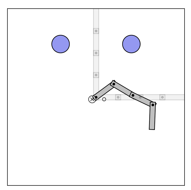
The simulated robot you'll be working with for this project is an articulated arm (picture shown on left). This arm has 4 degrees of freedom (DOFs).
Part 0 -- Download py_arm and install
Clone the py ARM github repo, and then pip install by following the directions in the README. You will then need to go to our Github classroom and download the codebase for PA2. You should then copy/paste your methods into the new rrt.py template.Part 1 -- Amend RRT to Implement Goal Biasing
In order for your existing RRT method to find a solution, it is necessary to sample a qrand configuration within the goal tolerance.
Imagine a configuration space with d dimensions. This space is discretized into 100 uniformly spaced cells. So, when d is 2, we have 10,000 cells. The formula for the volume of a hypercube is rd. The goal region consists of 4d cells.
Question: What is the probability of sampling qrand within the goal region? Solve for when d = 2, 3, 4, and 5.
Since RRT is commonly used to find paths in high-dimensional configuration spaces, this presents a real challenge. To address this, a common practice is to bias the exploration towards to the goal. Instead of selecting qrand randomly, every so often, assign qgoal as qrand. A common approach to this is to specify a goal_bias parameter which is in the range [0,1]. A random sample is then drawn within the main RRT loop, and when the random parameter is less than the goal_bias parameter, utilize qgoal as qrand. Implement this change and try different goal_bias parameters.Part 2 -- Amend RRT to Work with PyArm with 2 DOFs
This assignment includes a new rrt.py file. This contains some new methods and new import statements to utilize py-arm. You should follow these steps:
- Copy your rrt code into the rrt method (notice that the tree constructor is a little different, and thus, is included in the new rrt.py). This can include any helper methods you added to Tree and RRTNode.
- Run rrt_planner_arm.py file. This script takes a few parameters, but the defaults are OK for now. If all is OK with your RRT implementation, you should see a animation that shows the path of py-arm moving from qstart (fully extended to the right), to qgoal (fully extended up and down).
- Change RRT so that it computes the cost of the found path using the get_cost method within the Tree class.
- Verify there are no calls to numpy's seed function (we do not want the same pseudorandom sequence generated each time).
- cost of the solution in terms of path length (use get_cost from the Tree class)
- wallclock time for RRT to find the solution
- size of the RRT tree
Part 3 -- Try other Arms
This part of the PA is to study the variance in RRT's performance. Repeat the data collection from Part 1 (the cost, wallclock, and size of tree) for 30 runs with these three variants of the arm problem:- 3 DOFs
- 3 DOFs w/an additional obstacles at (20, 20) and (-40,50). You will need to modify the list passed to the ArmProblem constructor.
- 4 DOFs
- 5 DOF
Part 4 -- Reflection on A*
Now, think back to A*, ans these questions:- Imagine the grid for A* for the 4 DOF and 5 DOF problems. What grid discretization would you pick? How many cells are in the grid for each of these problems?
- Run the astar_planner_arm.py script and pass it --armDOFs=2. Record the wall clock time, path costs and expansions. Then run it for 3 and 4 DOFs. Compare and contrast the average runtimes and path costs for A* and the corresponding RRT problems solved earlier.
Part 5 -- Add an RRT* method
Amend rrt.py and complete the function named rrtstar
that takes the same arguments as rrt. It must implement the
RRT* algorithm as discussed in class and following the
pseudo-code from the lecture slides. Some highlights on the modifications
are listed below:
- Your method must continue to run after a solution is found, and thus, the tree must be grown until the tree_size specified is reached.
- After a solution is found, the program outputs the cost of the best solution and the size of the tree each time a node is added to the tree. The tree is always grown to the maxsize in RRT* since node additions can improve the quality of paths to qgoal.
- The code must wire qnew to the node in the neighborhood that is collision free and minimizes its cost (which may or may not be qnear). To identify the neighborhood, you can use 1.5 times the stepsize and utilize the within_delta method within spatial_map.py to identify the nodes that are in the neighborhood.
- After adding qnew, nodes in the neighborhood need to be evaluated to see if an edge can be added, and if so, will it lower the cost to the node. If both those conditions are true, the the node should be rewired so that qnew is its new parent.
Submitting
Your submission will be graded on the basis of code-quality, documentatation, and quality of your report.
Submissions will be graded according to the following rubric:
| Answer the questions about the probability of sampling qrand within the goal region for the different problems (d=2, 3, 4, and 5) | 10% |
| Augment rrt.py to provide the required stats for the analysis and goal biasing. The rrt_planner_arm.py file should enable you to experiment try different DOFs and goal biases. Create scripts rrt_dof2.py, rrt_dof3.py, rrt_dof3extra.py, rrt_dof4.py, and rrt_dof5.py that record the statistics you need for your analysis (which would include running the method 30 times). | 20% |
| Box plots showing the variance in terms of cost, run time, and tree size (1 whisker plot for each) for the 3 DOF, 3 DOF (w/2 additional obstacles), 4 DOF and 5 DOF problems (so, a total of 12 plots in total). These plots should be submitted in your written report (PDF format) and clearly labeled as to which experiment corresponds to which plot. | 10% |
| Answer to Part 4 (Questions on A* grid size and discretization). | 5% |
| Augment rrt.py to include RRT* method. Scripts to execute rrtstar 30 times on each DOF 2, DOF 3, DOF 3 w/extra obstacles, DOF 4, and DOF 5 problems, (script named rrtstar_dof2.py, rrtstar_dof3.py, rrtstar_dof3extra.py, etc). Scripts must output data that is used in the creation of the plots for path cost and runtime analysis. | 30% |
| Boxplots for runtime and path cost for the 30 runs for each problem ( 2 DOFs, 3 DOFs, 3 DOFs w/extra obstacles, 4 DOFS, and 5 DOFs). Plots to be included in the report. Report must include a short analysis (4 to 6 sentences) that discusses how RRT* scales for different DOFs and compare/constrast this to RRT and A*. | 15% |
| For a run of RRT* on the 4 DOF problem, plot of tree size (x-axis) and path cost (y-axis). Recall that because of the way RRT* rewires the tree, it is possible for the path cost to improve without adding a new that is closer to the goal. This plot must be within your submitted PDF. | 10% |