Your Problem

1 - Minimum Vertex Cover

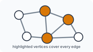
Given a simple undirected graph $G=(V,E)$, a vertex cover is a set $C\subseteq V$ such that every edge has at least one endpoint in $C$:

The optimization problem asks for a vertex cover of minimum size. Throughout this project, Minimum Vertex Cover is abbreviated MVC and uses the problem identifier minimum_vertex_cover (short command-line alias mvc).

Before implementing your algorithms, review the project-wide Program Interface and Input Files pages.

Graph assumptions

MVC instances use the shared course Graph representation.

• Vertices are numbered $0,1,\ldots,n-1$.
• Graphs are simple and undirected.
• Graphs need not be connected.
• Isolated vertices may appear.

MVC solution format

A solver returns one vertex cover:

{
  "size": 3,
  "vertices": [0, 2, 3]
}

vertices represents a set, so its order is not significant and duplicates are not permitted. size must equal len(vertices). If several minimum covers exist, any one of them is acceptable.

For example:

python src/solve.py example-01.txt \
    --problem mvc \
    --algorithm exhaustive

runs the MVC exhaustive solver through the common course driver.

Solution verifier

Your Checkpoint 1 implementation must provide:

from course.common.graph import Graph


def is_vertex_cover(graph: Graph, vertices: list[int], k: int) -> bool:
    ...

in:

src/student/problems/minimum_vertex_cover/verifier.py

This is the verifier for the decision version of MVC. It returns True exactly when all of the following hold:

1. vertices contains only valid graph vertices and contains no duplicates;
2. every edge has at least one endpoint in vertices; and
3. the certificate contains at most k vertices.

The verifier checks the supplied certificate and threshold. It does not determine whether the cover is minimum and must not call a solving algorithm. Gradescope may import and test the verifier independently of src/solve.py.

A direct implementation can convert the list to a set once and then scan all edges, giving polynomial running time.

Checkpoint 1 exhaustive baseline

Checkpoint 1 uses the project-wide complete-candidate enumeration model. For MVC:

1. try candidate sizes $k=0,1,2,\ldots$ from small to large;
2. for each $k$, enumerate every vertex subset of size $k$; and
3. test each completed subset with is_vertex_cover().

Once the first valid cover is found, it is optimal because every smaller candidate size has already been exhausted.

The Checkpoint 1 baseline should not reject partial subsets, branch on uncovered edges, prune, memoize, use dynamic programming, or use branch-and-bound. Those techniques belong to the improved exact algorithm.

The exhaustive solver must also record:

statistics["candidates"]

Increment this counter exactly once for each complete vertex subset that is actually tested as a candidate cover. Partial states and loop iterations that do not produce a tested complete subset are not candidates.

Checkpoint 2 improved exact search

MVC has a useful structural observation. If an edge $\{u,v\}$ is currently uncovered, every vertex cover must contain at least one of its endpoints. Therefore an exact search may branch into two subproblems:

include u
or
include v

and continue on the remaining uncovered edges. This can avoid enormous portions of the complete-subset search performed by the Checkpoint 1 baseline.

Additional exact improvements may include better edge/vertex selection, reduction rules, an incumbent solution, lower-bound pruning, memoization, or other justified techniques. These are examples rather than a mandated implementation. Your solver must remain exact and you must explain why any pruned work cannot contain a better solution.

Checkpoint 2 lower bound

MVC is a minimization problem, so the required polynomial-time bound is a lower bound:

from course.common.graph import Graph


def lower_bound(graph: Graph) -> int:
    ...

in:

src/student/problems/minimum_vertex_cover/bound.py

If the optimum is $OPT$, the returned value must always satisfy

One natural source of a lower bound is a maximal matching. The edges of a matching share no endpoints, and covering each matched edge requires selecting at least one distinct endpoint. Therefore the size of any matching is a valid lower bound on the minimum vertex-cover size. A greedily constructed maximal matching is polynomial-time and is sufficient as one possible design.

You are not required to use that particular bound. The returned value must be valid for every legal instance, polynomial-time computable, and sufficiently informative for the checkpoint tests.

Checkpoint 2 heuristic

heuristic1 must always return a valid cover and must run in polynomial time. It must also include a randomized component, perform multiple attempts or restarts, retain the best valid cover found so far, and reproduce the same result when run with the same --seed.

A single deterministic greedy construction followed immediately by return is not sufficient for heuristic1.

Course benchmark suites

The supplied MVC benchmark manifest is located at:

benchmarks/minimum_vertex_cover/manifest.json

Run the common experiment tool with, for example:

python tools/run_experiments.py --suite exact_frontier
python tools/run_experiments.py --suite quality_known
python tools/run_experiments.py --suite heuristic_scale
python tools/run_experiments.py --suite structure

Exact frontier

The exact-search frontier contains three known-optimum families:

• balanced complete bipartite graphs;
• disjoint star forests; and
• disjoint triangles.

The default local exact-frontier timeout is 15 minutes per algorithm/instance. After one algorithm times out on a member of a frontier family, larger members of that same family are skipped for that algorithm. Gradescope uses shorter safety ceilings; the local frontier is where you study when each exact method becomes impractical.

Heuristic scale

The scale suite uses bipartite graphs with certified optima at 500, 2,000, and 5,000 vertices. In each graph, one side of the bipartition is a cover of size $k$, while a matching of size $k$ proves that no smaller cover exists.

Structural experiment

The required structural family holds both size and optimum fixed:

• $n=300$;
• $OPT=120$.

The amount of additional cross-edge structure is changed to produce sparse, medium, and dense instances. This lets you investigate the effect of edge density without simultaneously changing the number of vertices or the known optimal cover size.

See:

benchmarks/minimum_vertex_cover/structure.md

for the construction and interpretation details.

PACE 2019 open challenge

After your assigned problem appears in project.json, run:

python tools/setup_project.py

For Minimum Vertex Cover, setup installs a curated 20-instance challenge set from the official PACE 2019 Vertex Cover Exact archive. The source archive is the PACE Track 1 dataset deposited on Zenodo (DOI 10.5281/zenodo.3368306).

The 20 instances were selected conservatively from the detailed result tables in Hespe, Lamm, Schulz, and Strash’s WeGotYouCovered report: for each selected row, none of the listed exact configurations solved the instance in the reported experiment, and the table therefore gives no minimum-cover value. The course records known_optimum = null rather than treating a feasible solution or an uncertified value as OPT.

The downloaded graphs are converted to the course’s 0-based simple-graph format and stored locally under:

benchmarks/minimum_vertex_cover/external/pace2019/instances/

They are ignored by Git. Run the collection with:

python tools/run_experiments.py --suite challenge_open

If your heuristic finds a cover of size $U$ and your lower-bound routine returns $L$, the evidence supports:

A better feasible cover narrows the upper end of that interval; it does not prove optimality unless a separate cited source establishes the exact minimum.

See Challenge Benchmarks and Leaderboards for the common challenge rules.

2 - Minimum Graph Coloring

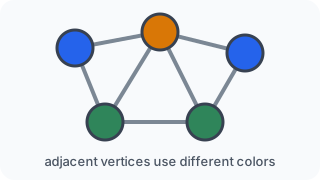
Given an undirected graph $G=(V,E)$, a proper vertex coloring assigns a color to every vertex such that no two adjacent vertices receive the same color.

More formally, if $c(v)$ denotes the color assigned to vertex $v$, then for every edge $(u,v) \in E$,

The goal of Minimum Graph Coloring is to find a proper coloring that uses the smallest possible number of colors. The minimum number of colors required to properly color a graph is called its chromatic number.

Throughout this specification, Minimum Graph Coloring is abbreviated MGC.

Your goal throughout the project will be to investigate algorithms involving graph colorings. The specific algorithmic tasks required at each stage are described in the corresponding checkpoint.

Before implementing your algorithms, review the project-wide Program Interface and Input Files specifications.

Graph Assumptions

MGC instances use simple, undirected graphs.

• Vertices are numbered consecutively beginning with 0: $V=\{0,1,\ldots,n-1\}$.
• Graphs are not necessarily connected.
• Isolated vertices may appear.
• Every vertex must be assigned exactly one color.

The standard unweighted graph formats and supplied input routines are described on the Input Files page.

Example

The same graph and its edge-list representation are shown side-by-side below.

The number in parentheses beside each vertex indicates its assigned color.

Example graph                                  example-01.txt

               1 (1)                               5 5
              /     \                               0 1
             /       \                              1 2
          0 (0)     2 (0)                           2 3
             \       /                              3 4
              \     /                               4 0
               4 (2) --- 3 (1)

This coloring uses three colors:

Every pair of adjacent vertices has a different color, so this is a valid coloring.

This graph is an odd cycle and cannot be properly colored using only two colors. Therefore, the coloring shown above is a minimum coloring and the chromatic number of the graph is 3.

For comparison, the assignment

is not a valid coloring because vertices 0 and 4 are adjacent and are both assigned color 0.

MGC Solution Format

MGC uses minimum_graph_coloring as its project-wide problem identifier.

The solution object contains the number of colors used and the color assigned to each vertex:

"solution": {
  "num_colors": 3,
  "colors": [0, 1, 0, 1, 2]
}

The entry colors[v] gives the color assigned to vertex $v$. Therefore, the colors list must contain exactly one entry for every vertex in the graph.

Color numbers begin with 0. If a solution uses $k$ colors, the colors must be numbered consecutively:

The actual numbers used as color labels have no special meaning. Only whether two vertices have the same or different colors matters.

num_colors must equal the number of distinct colors appearing in the colors list.

Using the common project interface,

python src/solve.py example-01.txt \
    --problem minimum_graph_coloring \
    --algorithm exhaustive

could produce:

{
  "problem": "minimum_graph_coloring",
  "algorithm": "exhaustive",
  "instance": "example-01",
  "solution": {
    "num_colors": 3,
    "colors": [0, 1, 0, 1, 2]
  },
  "statistics": {}
}

Your program is required to report only one minimum coloring. If an instance has multiple minimum colorings, any one of them is acceptable; your program does not need to enumerate all optimal solutions.

Different assignments of color numbers may represent equivalent colorings. For example, replacing every color 0 with color 1 and every color 1 with color 0 does not create a fundamentally different coloring.

Solution Verifier

Your Checkpoint 1 implementation must provide:

from course.common.graph import Graph


def is_valid_coloring(graph: Graph, colors: list[int], k: int) -> bool:
    ...

in:

src/student/problems/minimum_graph_coloring/verifier.py

This is the verifier for the decision version of Minimum Graph Coloring. It returns True exactly when colors is a proper coloring of graph that uses at most k distinct colors.

For the example graph:

is_valid_coloring(graph, [0, 1, 0, 1, 2], 3)   # True
is_valid_coloring(graph, [0, 1, 0, 1, 2], 2)   # False: uses 3 colors
is_valid_coloring(graph, [0, 1, 0, 1, 0], 3)   # False: edge (0,4) conflicts

A certificate must assign exactly one nonnegative integer color to every vertex. Adjacent vertices must receive different colors. The verifier does not need to require consecutive color labels; for example, [4,7,4,7,9] can be a valid certificate using three colors. Solver output, however, must normalize its labels to 0,1,...,k-1.

The verifier checks the supplied certificate and threshold. It does not determine whether the coloring is minimum and must not call a solving algorithm.

Gradescope may import and test is_valid_coloring() independently of src/solve.py.

Checkpoint 1 Exhaustive Baseline

Checkpoint 1 uses the project-wide complete-candidate enumeration model. For Minimum Graph Coloring, try k = 1, 2, 3, .... For each k, enumerate complete assignments of all n vertices to the k available colors. Each completed assignment is then tested with is_valid_coloring().

Once the first feasible k is found, that coloring is optimal because every smaller number of colors has already been exhausted.

The Checkpoint 1 baseline should not reject a coloring while it is still only partially assigned, choose the next vertex adaptively, prune impossible partial assignments, or use branch-and-bound. Those are the kinds of improvements explored beginning in Checkpoint 2.

Checkpoint 2 Improved Exact Search

A natural improved exact strategy assigns colors incrementally and rejects a partial coloring as soon as it creates a conflict. More sophisticated exact methods may choose the next vertex using degree or saturation information and may use bounds to avoid trying color counts that cannot succeed.

For example, a recursive search can maintain a partial color assignment and, for the next vertex, consider only colors not already used by its colored neighbors. This avoids generating many complete assignments that the Checkpoint 1 exhaustive baseline would generate and reject only at the end.

These are examples rather than required implementations. Your improved solver must remain exact and you must justify why any work it avoids cannot eliminate an optimal coloring.

Checkpoint 2 Lower Bound

Minimum Graph Coloring is a minimization problem, so the required polynomial-time bound is a lower bound on the chromatic number:

from course.common.graph import Graph


def lower_bound(graph: Graph) -> int:
    ...

in:

src/student/problems/minimum_graph_coloring/bound.py

If the optimum chromatic number is $OPT$, a valid result must satisfy

One useful source of lower bounds is a clique that you can find in polynomial time: if you find a clique of size $r$, then at least $r$ colors are required. The bound routine does not need to find a maximum clique; that would itself be an NP-hard problem. A greedily constructed clique, a detected triangle, or another polynomial-time argument can provide a valid lower bound.

You are not required to use a particular technique, but the returned value must be valid and computed in polynomial time.

Course Benchmark Suites

The supplied Minimum Graph Coloring benchmark manifest is located at:

benchmarks/minimum_graph_coloring/manifest.json

The required suites use the common experiment tool, for example:

python tools/run_experiments.py --suite exact_frontier
python tools/run_experiments.py --suite quality_known
python tools/run_experiments.py --suite heuristic_scale
python tools/run_experiments.py --suite structure

Exact frontier

The exact-search frontier contains three graph families with known chromatic numbers by construction:

• odd cycles — sparse graphs with chromatic number 3;
• complete graphs — K_n requires exactly n colors; and
• planted four-color graphs — each graph contains a K_4 but all other edges are placed between four known color classes, proving that the chromatic number is exactly 4.

The default local exact-frontier timeout is 15 minutes per algorithm/instance. After an algorithm times out on one member of a frontier family, larger members of that same family are skipped for that algorithm.

The Gradescope timeout is intentionally shorter. Gradescope is a bounded automated check; the Final Project exact-search frontier is where you investigate when your exact algorithm becomes impractical.

Heuristic quality and scale

The known-quality and scale suites use planted k-colorable graphs that also contain a K_k. Therefore their chromatic number is exactly k, even for the largest instances. The scale suite extends through 5,000 vertices.

Structural experiment

The required structural study holds both graph size and optimum fixed:

• $n=300$;
• $OPT=8$.

Each graph is built from eight planted color classes and contains an explicit K_8. Additional edges are added only between different color classes, so an 8-coloring always exists. The benchmark varies the probability of these additional cross-class edges, producing low-, medium-, and high-density graphs while keeping both n and the chromatic number fixed.

This lets you investigate whether edge density affects heuristic solution quality, runtime, variation across seeds, or the tightness of your lower bound without simultaneously changing graph size or the optimum.

See:

benchmarks/minimum_graph_coloring/structure.md

for the full description.

Open DIMACS/COLOR challenge

After your project has been assigned and assigned_problem has been set, run:

python tools/setup_project.py

For Minimum Graph Coloring, setup downloads a curated 20-instance open challenge from the established DIMACS/COLOR graph-coloring benchmark collections. The set includes long-standing hard DIMACS random graphs, eight real optical-network coloring instances, and two additional structured hard instances. The downloaded .col files are converted to the common Beyond Brute Force graph format and stored under:

benchmarks/minimum_graph_coloring/external/dimacs/instances/

Those downloaded graph files are ignored by Git. The tracked manifest preserves the original instance name, benchmark collection, download URL, citation, and any published reference value used by the course.

Run the challenge with:

python tools/run_experiments.py --suite challenge_open

For these challenge entries, known_optimum = null means that the course is not claiming a certified chromatic number. If your heuristic finds a valid coloring using U colors and your polynomial-time lower-bound routine returns L, then you may report

Some manifest entries also contain a published feasible coloring (best_known) or a published lower bound. Treat those values as references with the meaning stated in the manifest; do not call a best-known coloring optimal unless its cited source proves optimality.

3 - Maximum Clique

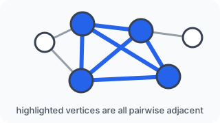
Given an undirected graph $G=(V,E)$, a clique is a subset of vertices $C \subseteq V$ in which every pair of distinct vertices is connected by an edge.

More formally, for every pair of distinct vertices $u,v \in C$,

The goal of Maximum Clique is to find a clique containing the largest possible number of vertices.

Throughout this specification, Maximum Clique is abbreviated MC.

Before implementing your algorithms, review the project-wide Program Interface and Input Files specifications.

Graph Assumptions

MC instances use simple, unweighted, undirected graphs.

• Vertices are numbered consecutively beginning with 0: $V=\{0,1,\ldots,n-1\}$.
• Graphs are not necessarily connected.
• Isolated vertices may appear.

The standard unweighted graph formats and supplied input routines are described on the Input Files page.

Example

The same graph and its edge-list representation are shown side-by-side below. Filled vertices are members of one maximum clique.

Example graph                                  example-01.txt

       ● 0 ------- ● 1                               5 6
           \       /                                 0 1
            \     /       ● = in the clique          0 2
              ● 2         ○ = not in the clique      1 2
            /     \                                  2 3
           /       \                                 2 4
       ○ 3 ------- ○ 4                               3 4

The filled vertices represent the clique

Every pair of vertices in $C$ is connected by an edge: $(0,1)$, $(0,2)$, and $(1,2)$ are all present.

This graph contains no clique of size 4, so $C$ is a maximum clique. The graph also contains another maximum clique, $\{2,3,4\}$.

For comparison, $\{0,1,3\}$ is not a clique because vertices 0 and 3 are not adjacent.

MC Solution Format

MC uses maximum_clique as its project-wide problem identifier. The short command-line alias is mc.

The solution dictionary contains the vertices in the reported clique and the size of that clique:

{
  "size": 3,
  "vertices": [0, 1, 2]
}

The vertices list represents a set. Its order is not significant. Duplicate vertices are not permitted, and size must equal the number of entries in the list.

Using the common project interface,

python src/solve.py example-01.txt \
    --problem mc \
    --algorithm exhaustive

could produce a solution containing $[0,1,2]$.

Your program is required to report only one maximum clique. If an instance has multiple maximum cliques, any one of them is acceptable; your program does not need to enumerate all optimal solutions.

Solution Verifier

Your Checkpoint 1 implementation must provide:

from course.common.graph import Graph


def is_clique(graph: Graph, vertices: list[int], k: int) -> bool:
    ...

in:

src/student/problems/maximum_clique/verifier.py

This is the verifier for the decision version of Maximum Clique. It returns True exactly when vertices forms a clique in graph containing at least k vertices.

For the example graph:

is_clique(graph, [0, 1, 2], 3)   # True
is_clique(graph, [0, 1, 2], 4)   # False
is_clique(graph, [0, 1, 3], 3)   # False: (0,3) is not an edge

A valid certificate must contain only vertices from the graph, with no duplicates, and every pair of distinct supplied vertices must be adjacent.

The verifier checks the supplied certificate. It does not determine whether that clique is maximum and must not call one of the solving algorithms.

Gradescope may import and test is_clique() independently of src/solve.py.

Checkpoint 1 Exhaustive Baseline

Checkpoint 1 uses the project-wide complete-candidate enumeration model. For Maximum Clique, a complete candidate is a subset of vertices.

A natural exact baseline considers candidate sizes from large to small, enumerates every subset of the current size, and sends each complete candidate to is_clique(). Once a valid candidate of size $k$ is found, it is optimal because every larger candidate size has already been exhausted.

The Checkpoint 1 baseline should not reject partial subsets, recursively grow only promising cliques, prune branches, or use branch-and-bound. Those are the kinds of improvements explored beginning in Checkpoint 2.

Checkpoint 2 Improved Exact Search

A natural improved exact strategy builds a clique incrementally. If C is the clique currently being constructed and P is the set of vertices that may still be added, every vertex in P must be adjacent to every vertex already in C.

After choosing a vertex v from P, a recursive search can continue with:

C' = C ∪ {v}
P' = (P - {v}) ∩ neighbors(v)

This immediately discards vertices that cannot extend the current clique. A simple branch-and-bound rule can also stop whenever the current clique plus all remaining candidates cannot improve the best clique already found.

These are examples rather than required implementations; your improved solver must remain exact and you must justify why any work it avoids cannot eliminate an optimal solution.

Checkpoint 2 Upper Bound

Maximum Clique is a maximization problem, so the required polynomial-time bound is an upper bound on the optimal clique size:

from course.common.graph import Graph


def upper_bound(graph: Graph) -> int:
    ...

in:

src/student/problems/maximum_clique/bound.py

If the optimum is $OPT$, a valid result must satisfy

There are several possible polynomial-time upper bounds. For example, $\Delta(G)+1$ is valid because a vertex in a clique of size $k$ has at least $k-1$ neighbors. A proper coloring also gives an upper bound because a clique can contain at most one vertex of each color.

You are not required to use either particular bound, but the returned value must be valid and computed in polynomial time.

Course Benchmark Suites

The supplied Maximum Clique benchmark manifest is located at:

benchmarks/maximum_clique/manifest.json

The required suites use the common experiment tool, for example:

python tools/run_experiments.py --suite exact_frontier
python tools/run_experiments.py --suite quality_known
python tools/run_experiments.py --suite heuristic_scale
python tools/run_experiments.py --suite structure

Exact frontier

The exact-search frontier contains three families with known optima:

• balanced complete bipartite graphs — the maximum clique has size 2, so a large fraction of larger subsets must be rejected by the exhaustive baseline;
• complete multipartite graphs with parts of size 3 — a maximum clique contains exactly one vertex from each part; and
• two disconnected equal cliques — dense local structure combined with a complete absence of edges between the two components.

The default local exact-frontier timeout is 15 minutes per algorithm/instance. After an algorithm times out on one member of a frontier family, larger members of that same family are skipped for that algorithm.

The Gradescope timeout is intentionally shorter. Gradescope is a bounded automated check; the Final Project exact-search frontier is where you investigate when your exact algorithm becomes impractical.

Heuristic scale

The scale suite uses sparse graphs containing a planted clique together with many independent distractor vertices. Required instances extend to 5,000 vertices while retaining a known optimum by construction.

Structural experiment

The required structural study holds both graph size and optimum fixed:

• $n=300$;
• $OPT=10$.

Every instance is a complete 10-partite graph. The part-size distribution is changed to vary edge density while preserving the exact optimum. This lets you investigate whether density affects heuristic quality, runtime, variation across seeds, or the tightness of your upper bound without simultaneously changing problem size or the optimal clique size.

See:

benchmarks/maximum_clique/structure.md

for the full description.

Open SNAP challenge

After your problem assignment appears in project.json, install the external challenge data once with:

python tools/setup_project.py

For Maximum Clique, setup installs a curated 20-instance SNAP social-network collection containing undirected Facebook, Deezer, Twitch, GitHub, and Facebook ego-network graphs. The actual graph files are downloaded locally under:

benchmarks/maximum_clique/external/snap/instances/

and are intentionally ignored by Git. The tracked manifest preserves the original SNAP source page, source filename or archive member, citation, and download information for every instance. Source files are normalized to a simple undirected graph: self-loops are removed and repeated/reversed edges are collapsed. When that changes the edge count, the manifest retains SNAP’s published source count separately from the installed simple-graph count.

Run the collection with:

python tools/run_experiments.py --suite challenge_open

These are open challenge instances: the course does not claim a proven optimum, so the manifest records known_optimum = null. If your heuristic finds a valid clique of size $L$ and your polynomial-time bound returns $U$, then you may report only

Your clique establishes a feasible lower bound. A larger clique found by another team is another feasible lower bound, not proof of optimality.

4 - Traveling Salesperson

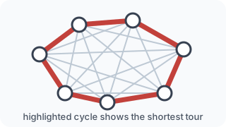
Given a weighted graph $G=(V,E)$, a tour is a cycle that visits every vertex exactly once before returning to its starting vertex.

If a tour visits the vertices in the order

then its total cost is the sum of the weights of the edges used by the tour:

The goal of the Traveling Salesperson Problem is to find a tour with the smallest possible total cost.

Throughout this specification, Traveling Salesperson Problem is abbreviated TSP.

Your goal throughout the project will be to investigate algorithms involving TSP tours. The specific algorithmic tasks required at each stage are described in the corresponding checkpoint.

Before implementing your algorithms, review the project-wide Program Interface and Input Files specifications.

Graph Assumptions

TSP instances use weighted, undirected, complete graphs.

• Vertices are numbered consecutively beginning with 0: $V=\{0,1,\ldots,n-1\}$.
• Every pair of distinct vertices is connected by exactly one edge.
• Edge weights are nonnegative integers.
• Because the graph is undirected, $w(u,v)=w(v,u)$.
• A valid tour visits every vertex exactly once and then returns to its starting vertex.

The weighted graph format and supplied input routines are described on the Input Files page.

Example

Consider the following complete weighted graph instance:

example-01.txt

4 6
0 1 10
0 2 15
0 3 20
1 2 35
1 3 25
2 3 30

The first line indicates that the graph contains four vertices and six edges. Each remaining line gives two endpoints followed by the weight of that edge.

One tour is

Its total cost is

For this instance, the three distinct tours beginning at vertex 0, ignoring reversal, have costs:

Therefore, the tour $[0,1,3,2,0]$ is a minimum-cost tour.

For comparison,

is not a valid TSP tour because vertex 3 is never visited.

TSP Solution Format

TSP uses traveling_salesperson as its project-wide problem identifier.

The solution object contains the reported tour and its total cost:

"solution": {
  "cost": 80,
  "tour": [0, 1, 3, 2, 0]
}

The order of vertices in tour is significant.

For a graph containing $n$ vertices, the tour list must contain exactly $n+1$ entries. The first and last entries must be the same, and every graph vertex must appear exactly once among the first $n$ entries.

cost must equal the sum of the weights of the $n$ edges traversed by the tour.

The starting vertex is not significant. For example,

and

represent the same cycle. Because the graph is undirected, traversing the cycle in the opposite direction also represents the same tour.

Using the common project interface,

python src/solve.py example-01.txt \
    --problem tsp \
    --algorithm exhaustive

could produce:

{
  "problem": "traveling_salesperson",
  "algorithm": "exhaustive",
  "instance": "example-01",
  "solution": {
    "cost": 80,
    "tour": [0, 1, 3, 2, 0]
  },
  "statistics": {}
}

Your program is required to report only one minimum-cost tour. If an instance has multiple minimum-cost tours, any one of them is acceptable; your program does not need to enumerate all optimal solutions.

Decision-Problem Verifier

The verifier you implement corresponds directly to the polynomial-time certificate verifier for the decision version of TSP:

Given a weighted graph $G$ and a threshold $k$, does $G$ contain a tour whose total cost is at most $k$?

The proposed tour is the certificate. Your implementation must provide:

from course.common.weighted_graph import WeightedGraph

def is_valid_tour(graph: WeightedGraph, tour: list[int], k: int) -> bool:
    ...

in:

src/student/problems/traveling_salesperson/verifier.py

Two WeightedGraph interface details are especially useful when implementing this verifier:

n = graph.num_vertices       # integer attribute -- no parentheses
w = graph.weight(u, v)       # weight of edge (u, v)

Thus, for example, iterate over the vertices with range(graph.num_vertices) rather than calling graph.num_vertices(). The complete shared weighted-graph interface is documented on the Program Interface page.

The verifier must return True exactly when:

1. tour is a valid TSP tour of graph; and
2. the total cost of that tour is at most k.

The verifier must compute the tour cost from graph and tour; it must not trust a separately reported solution cost.

For the example graph, [0, 1, 3, 2, 0] has cost 80. Therefore:

is_valid_tour(graph, [0, 1, 3, 2, 0], 80)  # True
is_valid_tour(graph, [0, 1, 3, 2, 0], 79)  # False

A malformed tour must still be rejected regardless of the threshold:

is_valid_tour(graph, [0, 1, 2, 0], 1000)    # False: vertex 3 is missing

The verifier does not determine whether the tour is minimum-cost. It checks whether the supplied certificate proves a YES answer for the particular decision threshold k, and it must run in polynomial time without calling one of the solving algorithms.

Gradescope may import is_valid_tour() directly and test both tour feasibility and the threshold condition independently of src/solve.py.

Checkpoint 2 Bound Function

TSP is a minimization problem, so the required bound is a lower bound on the minimum tour cost. Implement:

from course.common.weighted_graph import WeightedGraph

def lower_bound(graph: WeightedGraph) -> int | float:
    ...

in:

src/student/problems/traveling_salesperson/bound.py

The function must run in polynomial time and never return a value larger than the true optimal tour cost. An MST-based lower bound is one natural design to consider during Checkpoint 2. Teams may propose a different valid polynomial-time bound during the Early Project Review.

The same bound may be reused inside an improved exact branch-and-bound solver, but the experiment framework also calls it independently so that it can be used to evaluate heuristic solutions when OPT is unavailable.

Course Benchmark Suites

The project template contains TSP benchmark suites under:

benchmarks/traveling_salesperson/

The required suites are designed around different experimental questions:

• readiness checks the Checkpoint 2 interfaces on small instances;
• exact_frontier compares exhaustive and improved exact search over increasing sizes and three different edge-weight structures;
• quality_known evaluates early heuristic and bound quality where OPT is known;
• heuristic_scale checks heuristic behavior on coordinate-backed instances far beyond the practical exact-search range; and
• structure holds n fixed while comparing uniform Euclidean, clustered Euclidean, and non-geometric random-weight instances.

For randomized heuristics, the course runner uses several fixed seeds and preserves every run. This allows the Final Project to examine variation in both solution value and running time instead of drawing conclusions from one lucky or unlucky run.

Large coordinate-backed instances

Large Euclidean TSP benchmarks are stored as coordinates rather than as an explicit list of all $\binom{n}{2}$ weighted edges. Student code still receives the normal course WeightedGraph and calls:

graph.weight(u, v)

to obtain the integer edge weight. Students do not parse TSPLIB files or compute TSPLIB rounding themselves.

External leaderboard and open-challenge instances

The benchmark manifest also defines public TSP challenges from the University of Waterloo National and VLSI TSP collections.

• leaderboard_known contains National TSP instances whose optimal tour values have been proven. These can be scored by percentage gap from OPT.
• reach_known contains still larger proven-optimal National TSP instances.
• reach_open contains two very large open National TSP instances with a published best-known tour and certified lower bound.
• challenge_open is the common 20-instance open VLSI challenge, ranging from 14,233 to 38,478 cities. Waterloo lists every selected instance as open and publishes a best-known tour for each. The first six selected instances also have a published Concorde lower bound.

After your assigned problem is recorded in project.json, install the external files with the same setup command used by every problem track:

python tools/setup_project.py

Then run the common open challenge with:

python tools/run_experiments.py --suite challenge_open

For an open instance, report a gap to the published best-known tour, not a gap to OPT. A published lower bound, when available, is recorded separately. When Waterloo does not publish a lower bound, your team’s required polynomial- time lower-bound routine supplies the certified lower side of the interval.

For the known-OPT leaderboard, each instance is run under the same fixed course seeds. The recommended scoreboard score is the median percentage gap to OPT for each instance, averaged equally across the leaderboard instances. Lower is better. This reduces the influence of one unusually lucky randomized run. The best tour found and runtime summaries are reported separately.

See the Benchmark Suites page and benchmarks/traveling_salesperson/README.md in the repository for the complete suite definitions.

5 - Longest Path

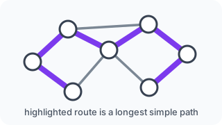
Given an undirected graph $G=(V,E)$, a simple path is a sequence of vertices

such that every consecutive pair of vertices is connected by an edge and no vertex appears more than once.

More formally,

for every $0 \le i < k$, and the vertices $v_0,v_1,\ldots,v_k$ are all distinct.

The length of a path is the number of edges it contains. Therefore, the path above has length $k$.

The goal of Longest Path is to find a simple path containing the largest possible number of edges.

Throughout this specification, Longest Path is abbreviated LP.

Before implementing your algorithms, review the project-wide Program Interface and Input Files specifications.

Graph Assumptions

LP instances use simple, unweighted, undirected graphs.

• Vertices are numbered consecutively beginning with 0: $V=\{0,1,\ldots,n-1\}$.
• Graphs are not necessarily connected.
• Isolated vertices may appear.
• A path may begin and end at any vertices in the graph.
• A vertex may appear at most once in a valid path.

The standard unweighted graph formats and supplied input routines are described on the Input Files page.

Example

The same graph and its edge-list representation are shown side-by-side below.

Example graph                                  example-01.txt

0 ------- 1 ------- 2 ------- 3                    5 5
           \       /                               0 1
            \     /                                1 2
              4                                    2 3
                                                   1 4
                                                   2 4

One valid path is

It uses four edges:

Because the graph contains five vertices, no simple path can contain more than four edges. Therefore, this path is a longest path.

For comparison,

is also a valid path, but it has length 3 and is therefore not optimal for this instance.

The sequence

is not a valid simple path because vertex 1 appears more than once.

LP Solution Format

LP uses longest_path as its project-wide problem identifier. The short command-line alias is lp.

The solution dictionary contains the vertices in the reported path and its length:

{
  "length": 4,
  "vertices": [0, 1, 4, 2, 3]
}

The vertices list gives the vertices in path order. Therefore, unlike a set of vertices, the order of this list is significant.

No vertex may appear more than once. Consecutive entries in the list must be connected by an edge in the graph.

For a nonempty path,

A path consisting of a single vertex is valid and has length 0.

Using the common project interface,

python src/solve.py example-01.txt \
    --problem lp \
    --algorithm exhaustive

could produce a solution containing the path shown above.

Your program is required to report only one longest path. If an instance has multiple longest paths, any one of them is acceptable; your program does not need to enumerate all optimal solutions.

A path and the same path written in reverse order represent the same undirected path. For example,

and

are equivalent solutions.

Solution Verifier

Your Checkpoint 1 implementation must provide:

from course.common.graph import Graph


def is_valid_path(graph: Graph, vertices: list[int], k: int) -> bool:
    ...

in:

src/student/problems/longest_path/verifier.py

This is the verifier for the decision version of Longest Path. It returns True exactly when vertices is a valid simple path in graph whose length is at least k.

For the example graph:

is_valid_path(graph, [0, 1, 4, 2, 3], 4)   # True
is_valid_path(graph, [0, 1, 4, 2, 3], 5)   # False
is_valid_path(graph, [0, 1, 4, 1, 2], 3)   # False: repeated vertex
is_valid_path(graph, [0, 4, 2], 2)         # False: (0,4) is not an edge

The verifier checks the supplied certificate. It does not determine whether that path is optimal and must not call one of the solving algorithms.

Gradescope may import and test is_valid_path() independently of src/solve.py.

Checkpoint 1 Exhaustive Baseline

Checkpoint 1 uses the project-wide complete-candidate enumeration model. For Longest Path, a complete candidate is an ordered sequence of distinct vertices.

A natural exact baseline considers longer candidate sequences before shorter ones and sends each complete candidate to is_valid_path(). Once a valid candidate of a given length is found, that path is optimal because all longer candidate lengths have already been exhausted.

The Checkpoint 1 baseline should not use recursive path extension, fail-early rejection of partial candidates, branch-and-bound, or other pruning techniques. Those are precisely the kinds of improvements explored beginning in Checkpoint 2.

Checkpoint 2 Upper Bound

Longest Path is a maximization problem, so the required polynomial-time bound is an upper bound on the optimal path length:

from course.common.graph import Graph


def upper_bound(graph: Graph) -> int:
    ...

in:

src/student/problems/longest_path/bound.py

If the optimum is $OPT$, a valid result must satisfy

A bound may be loose, but it should provide useful information beyond blindly returning a very large number. The public tests include disconnected graphs so that you can test whether your bound takes basic graph structure into account.

Course Benchmark Suites

The supplied Longest Path benchmark manifest is located at:

benchmarks/longest_path/manifest.json

The required suites are run with the common experiment tool, for example:

python tools/run_experiments.py --suite exact_frontier
python tools/run_experiments.py --suite quality_known
python tools/run_experiments.py --suite heuristic_scale
python tools/run_experiments.py --suite structure
python tools/run_experiments.py --suite challenge_open

Exact frontier

The exact-search frontier contains three families with known optima:

• three-arm trees — sparse graphs with very limited valid path extensions;
• imbalanced complete bipartite graphs — connected graphs with many choices but no Hamiltonian path when the two parts differ by more than one; and
• two disconnected cliques — dense local structure combined with a global connectivity restriction.

The default local exact-frontier timeout is 15 minutes per algorithm/instance. After an algorithm times out on one member of a frontier family, larger members of that same family are skipped for that algorithm.

The Gradescope timeout is intentionally shorter. Gradescope is a bounded automated check; the Final Project exact-search frontier is where you investigate when your exact algorithm becomes impractical.

Structural experiment

The required structural study holds the graph size fixed at 300 vertices and varies the probability of adding extra edges. Every instance contains a hidden, randomly labeled Hamiltonian path, so the optimum is always 299. This lets you study the effect of edge density without simultaneously changing graph size or the optimal objective value.

See:

benchmarks/longest_path/structure.md

for the full description.

Open challenge benchmarks

After your problem has been assigned, run the project setup command once:

python tools/setup_project.py

For Longest Path, setup installs a curated collection of 20 undirected network instances from the Stanford Large Network Dataset Collection (SNAP) under:

benchmarks/longest_path/external/snap/instances/

The collection includes collaboration, social, email-communication, Internet Autonomous-System, and Twitch friendship networks. The tracked manifest records the original SNAP instance name, source page, citation, graph size, and download information for every benchmark.

These instances form the optional challenge_open suite. The course deliberately records known_optimum = null for them: the manifest is not claiming a proven longest-path optimum. Use your polynomial-time upper bound together with the best valid path you find to report an interval

where $|P|$ is the objective value of your valid path and $U$ is your valid upper bound. You may compare your best feasible path with a class or published best-known value when one is available, but do not describe such a value as optimal without a proof of optimality.

The source SNAP graphs in this collection are undirected. Installation converts their edge lists to the course graph format; it does not turn directed data into undirected data.