This is the multi-page printable view of this section. Click here to print.
Projects
1 - Beyond Brute Force
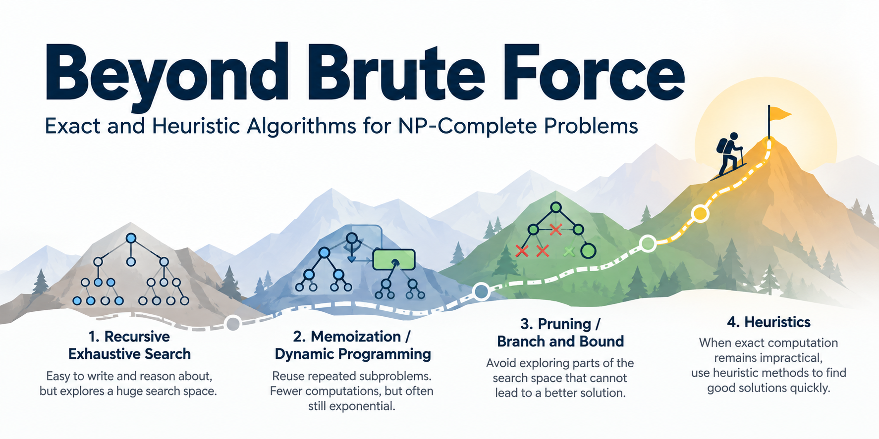
Overview
Beyond Brute Force is an integrative algorithms project in which each team studies one NP-complete optimization problem from theory through implementation and experimentation.
Over three weeks, you will build a straightforward exact baseline, develop improved exact and heuristic approaches, and use experiments to understand where the different methods succeed or struggle.
A useful way to think about the project is:
Week 1: Understand your problem, build the exhaustive baseline, and plan what comes next.
Week 2: Make the algorithms substantially better.
Week 3: Find out how good the algorithms actually are.
Start Here
If your team has not yet received an assigned problem, begin with Getting Started.
After your project is assigned, proceed to Checkpoint 1: Foundation to create your team repository and begin the algorithmic work.
Project Roadmap
| Stage | Goal | Points |
|---|---|---|
| Getting Started / Project Selection | Form your team, review the problem definitions, and submit three ranked project preferences through Gradescope. | 5 |
| Checkpoint 1: Foundation | Create the shared repository, configure the assigned problem, build and validate the exhaustive baseline, and plan what follows. | 25 |
| Early Project Review | Demonstrate individual understanding and team progress, identify problems early, and leave with concrete next steps for the major implementation work. | 10 |
| Checkpoint 2: Improved Algorithms | Implement and validate the bound, improved exact algorithm, and first heuristic. | 30 |
| Final Project | Experiment across benchmarks and challenges, determine what the algorithms can and cannot do, and synthesize the results. | 30 |
| Total | 100 |
Project Problems
Each team studies one of five NP-complete optimization problems. The diagrams below show the kind of solution each problem asks you to find.
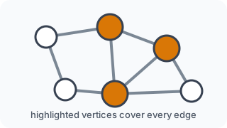 Minimum Vertex Cover
Choose as few vertices as possible to cover every edge.
Minimum Vertex Cover
Choose as few vertices as possible to cover every edge.
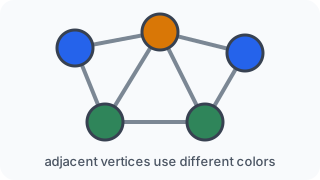 Minimum Graph Coloring
Color the vertices using as few colors as possible.
Minimum Graph Coloring
Color the vertices using as few colors as possible.
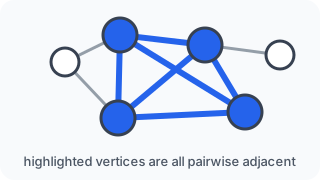 Maximum Clique
Find the largest set of pairwise adjacent vertices.
Maximum Clique
Find the largest set of pairwise adjacent vertices.
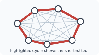 Traveling Salesperson
Find a shortest tour that visits every city exactly once.
Traveling Salesperson
Find a shortest tour that visits every city exactly once.
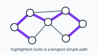 Longest Path
Find a longest simple path through the graph.
Longest Path
Find a longest simple path through the graph.
Teams and Shared Responsibility
Teams normally consist of two or three students; instructor-approved individual projects are permitted. Primary responsibility for one algorithm does not mean exclusive responsibility: every team member must understand the assigned problem, the verifier, and the major ideas used by the team.
The Early Project Review includes a short individual understanding check so that misconceptions can be corrected before the major implementation work of Week 2.
1.1 - Start Here
Begin with Getting Started to form your team, review the problem definitions, and submit three ranked project preferences on Gradescope. After the instructor assigns projects, follow Checkpoint 1 for Classroom 50 repository creation. The Learning Objectives page describes the project-wide goals and terminology.
1.1.1 - Getting Started
Goal: Form your team and submit your three ranked project preferences.
Points: 5 · Submission: Gradescope
Project Selection comes before Checkpoint 1. Follow the four steps below in order.
1. Form your team
Work in a team of two or three students, and choose a team name. Students who have instructor approval to work individually may submit as a one-person team. You will need the name of every team member for your submission.
2. Select your preferred problems
Read the five problem definitions before making your choices. Discuss them with your teammates and rank three distinct projects from most preferred (1) to least preferred (3). You are selecting preferences; you are not choosing your final assigned problem.
| Problem | Identifier for project_preferences |
|---|---|
| Traveling Salesperson | traveling_salesperson |
| Minimum Graph Coloring | minimum_graph_coloring |
| Minimum Vertex Cover | minimum_vertex_cover |
| Longest Path | longest_path |
| Maximum Clique | maximum_clique |
3. Complete the JSON file
Download the following files (also available with the Gradescope assignment):
Open it in a plain-text editor and fill in:
team_name: your team name (individual students should also choose a name);team_members: exactly one entry per student, each containing only anamefield;project_preferences: your three different project identifiers, ordered from first choice to third choice;assigned_problem: leave as the empty string ("") until your assignment is announced.
The starter file has two blank name entries. Adjust the team_members array to match your actual team:
- One student (instructor-approved): delete one of the two name entries, including the extra comma. Keep just one
{"name": "..."}object. - Two students: fill in the two existing name entries.
- Three students: add a third
{"name": "..."}object after the second, separated by a comma. The example below shows the required syntax.
Example: three students
{
  "team_name": "Graph Gurus",
  "team_members": [
    {"name": "Ada Example"},
    {"name": "Grace Example"},
    {"name": "Edsger Example"}
  ],
  "project_preferences": [
    "minimum_vertex_cover",
    "maximum_clique",
    "traveling_salesperson"
  ],
  "assigned_problem": ""
}
Check your file locally by placing check_project_selection.py beside project.json and running:
python3 check_project_selection.py
The checker prints PASS when the file is formatted correctly. It uses the same validation rules as the Gradescope autograder.
4. Submit on Gradescope
BBF - Problem and Group Selection
Open BBF - Problem and Group Selection on Gradescope. One student uploads project.json directly. For teams of two or three, include all teammates in the Gradescope group submission. Review the automatic feedback and resubmit if necessary before the deadline.
Submission checklist
- We have a team name and the names of every student (one student only when approved by the instructor).
- We ranked three distinct projects using the required identifiers.
-
assigned_problemis"". - The file is named
project.jsonand the local checker reportsPASS. - We submitted on Gradescope and included all teammates in the group submission, when applicable.
Grading (5 points)
| Component | Points | Assessment |
|---|---|---|
| Team information | 2 | Team name and 1–3 distinct student names |
| Ranked preferences | 2 | Exactly three distinct valid problems |
| Submission format | 1 | Required JSON fields and blank assigned_problem |
| Total | 5 |
4. The instructor assigns your project
The instructor will review the class’s ranked preferences, assign one of the five projects to each team or individual, and announce the assignments. Preferences are not guaranteed.
After your project is assigned, you will receive instructions for creating your shared repository through Classroom 50 as part of Checkpoint 1: Foundation. Do not create a project repository during Project Selection.
1.1.2 - Learning Objectives
By completing Beyond Brute Force, you should be able to:
- explain the relationship between an NP-complete decision problem and its optimization version;
- identify what constitutes a feasible solution and explain how a proposed solution can be verified efficiently;
- implement and analyze a straightforward exhaustive exact algorithm;
- reason about the state of an exact search and whether repeated subproblems are present;
- improve exact computation using an appropriate algorithm-design technique while preserving optimality;
- construct and justify a valid polynomial-time bound for an optimization problem;
- design and evaluate a polynomial-time heuristic for instances where exact computation becomes impractical;
- use reproducible randomized experiments and best-so-far behavior to evaluate heuristic approaches;
- compare heuristic results with known optima when available and with valid bounds or best-known solutions when OPT is unknown;
- perform controlled experiments across a collection of problem instances;
- identify input characteristics that affect computational effort or solution quality; and
- communicate algorithmic conclusions using appropriately qualified experimental evidence.
Key terminology
The theoretical portion of this project focuses on the decision version of your problem, while the programming and experimental portions focus on the corresponding optimization version.
- An exact algorithm is guaranteed to return an optimal solution when it terminates.
- An improved exact algorithm is still exact, but reduces the computation performed by the exhaustive baseline.
- A bound is an efficiently computed value guaranteed to lie on the appropriate side of the optimum.
- A heuristic algorithm returns a valid solution but does not necessarily guarantee optimality. For this project, heuristics must run in polynomial time so they can scale beyond the practical range of exact computation.
The checkpoint pages translate these project-wide objectives into concrete work for each stage.
1.2 - Your Problem
Use the specification for your assigned problem throughout the project. Each guide defines the solution format, decision verifier, exhaustive baseline, required bound, and problem-specific algorithm guidance.
1.2.1 - Minimum Vertex Cover
Given a simple undirected graph , a vertex cover is a set such that every edge has at least one endpoint in :
The optimization problem asks for a vertex cover of minimum size. Throughout
this project, Minimum Vertex Cover is abbreviated MVC and uses the problem
identifier minimum_vertex_cover (short command-line alias mvc).
Before implementing your algorithms, review the project-wide Program Interface and Input Files pages.
Graph assumptions
MVC instances use the shared course Graph representation.
- Vertices are numbered .
- Graphs are simple and undirected.
- Graphs need not be connected.
- Isolated vertices may appear.
MVC solution format
A solver returns one vertex cover:
{
  "size": 3,
  "vertices": [0, 2, 3]
}
vertices represents a set, so its order is not significant and duplicates are
not permitted. size must equal len(vertices). If several minimum covers
exist, any one of them is acceptable.
For example:
python src/solve.py example-01.txt \
    --problem mvc \
    --algorithm exhaustive
runs the MVC exhaustive solver through the common course driver.
Solution verifier
Your Checkpoint 1 implementation must provide:
from course.common.graph import Graph


def is_vertex_cover(graph: Graph, vertices: list[int], k: int) -> bool:
    ...
in:
src/student/problems/minimum_vertex_cover/verifier.py
This is the verifier for the decision version of MVC. It returns True
exactly when all of the following hold:
verticescontains only valid graph vertices and contains no duplicates;- every edge has at least one endpoint in
vertices; and - the certificate contains at most
kvertices.
The verifier checks the supplied certificate and threshold. It does not
determine whether the cover is minimum and must not call a solving algorithm.
Gradescope may import and test the verifier independently of src/solve.py.
A direct implementation can convert the list to a set once and then scan all edges, giving polynomial running time.
Checkpoint 1 exhaustive baseline
Checkpoint 1 uses the project-wide complete-candidate enumeration model. For MVC:
- try candidate sizes from small to large;
- for each , enumerate every vertex subset of size ; and
- test each completed subset with
is_vertex_cover().
Once the first valid cover is found, it is optimal because every smaller candidate size has already been exhausted.
The Checkpoint 1 baseline should not reject partial subsets, branch on uncovered edges, prune, memoize, use dynamic programming, or use branch-and-bound. Those techniques belong to the improved exact algorithm.
The exhaustive solver must also record:
statistics["candidates"]
Increment this counter exactly once for each complete vertex subset that is actually tested as a candidate cover. Partial states and loop iterations that do not produce a tested complete subset are not candidates.
Checkpoint 2 improved exact search
MVC has a useful structural observation. If an edge is currently uncovered, every vertex cover must contain at least one of its endpoints. Therefore an exact search may branch into two subproblems:
include u
or
include v
and continue on the remaining uncovered edges. This can avoid enormous portions of the complete-subset search performed by the Checkpoint 1 baseline.
Additional exact improvements may include better edge/vertex selection, reduction rules, an incumbent solution, lower-bound pruning, memoization, or other justified techniques. These are examples rather than a mandated implementation. Your solver must remain exact and you must explain why any pruned work cannot contain a better solution.
Checkpoint 2 lower bound
MVC is a minimization problem, so the required polynomial-time bound is a lower bound:
from course.common.graph import Graph


def lower_bound(graph: Graph) -> int:
    ...
in:
src/student/problems/minimum_vertex_cover/bound.py
If the optimum is , the returned value must always satisfy
One natural source of a lower bound is a maximal matching. The edges of a matching share no endpoints, and covering each matched edge requires selecting at least one distinct endpoint. Therefore the size of any matching is a valid lower bound on the minimum vertex-cover size. A greedily constructed maximal matching is polynomial-time and is sufficient as one possible design.
You are not required to use that particular bound. The returned value must be valid for every legal instance, polynomial-time computable, and sufficiently informative for the checkpoint tests.
Checkpoint 2 heuristic
heuristic1 must always return a valid cover and must run in polynomial time.
It must also include a randomized component, perform multiple attempts or
restarts, retain the best valid cover found so far, and reproduce the same
result when run with the same --seed.
A single deterministic greedy construction followed immediately by return is
not sufficient for heuristic1.
Course benchmark suites
The supplied MVC benchmark manifest is located at:
benchmarks/minimum_vertex_cover/manifest.json
Run the common experiment tool with, for example:
python tools/run_experiments.py --suite exact_frontier
python tools/run_experiments.py --suite quality_known
python tools/run_experiments.py --suite heuristic_scale
python tools/run_experiments.py --suite structure
Exact frontier
The exact-search frontier contains three known-optimum families:
- balanced complete bipartite graphs;
- disjoint star forests; and
- disjoint triangles.
The default local exact-frontier timeout is 15 minutes per algorithm/instance. After one algorithm times out on a member of a frontier family, larger members of that same family are skipped for that algorithm. Gradescope uses shorter safety ceilings; the local frontier is where you study when each exact method becomes impractical.
Heuristic scale
The scale suite uses bipartite graphs with certified optima at 500, 2,000, and 5,000 vertices. In each graph, one side of the bipartition is a cover of size , while a matching of size proves that no smaller cover exists.
Structural experiment
The required structural family holds both size and optimum fixed:
- ;
- .
The amount of additional cross-edge structure is changed to produce sparse, medium, and dense instances. This lets you investigate the effect of edge density without simultaneously changing the number of vertices or the known optimal cover size.
See:
benchmarks/minimum_vertex_cover/structure.md
for the construction and interpretation details.
PACE 2019 open challenge
After your assigned problem appears in project.json, run:
python tools/setup_project.py
For Minimum Vertex Cover, setup installs a curated 20-instance challenge set
from the official PACE 2019 Vertex Cover Exact archive. The source archive is
the PACE Track 1 dataset deposited on Zenodo (DOI 10.5281/zenodo.3368306).
The 20 instances were selected conservatively from the detailed result tables in
Hespe, Lamm, Schulz, and Strash’s WeGotYouCovered report: for each selected row,
none of the listed exact configurations solved the instance in the reported
experiment, and the table therefore gives no minimum-cover value. The course
records known_optimum = null rather than treating a feasible solution or an
uncertified value as OPT.
The downloaded graphs are converted to the course’s 0-based simple-graph format and stored locally under:
benchmarks/minimum_vertex_cover/external/pace2019/instances/
They are ignored by Git. Run the collection with:
python tools/run_experiments.py --suite challenge_open
If your heuristic finds a cover of size and your lower-bound routine returns , the evidence supports:
A better feasible cover narrows the upper end of that interval; it does not prove optimality unless a separate cited source establishes the exact minimum.
See Challenge Benchmarks and Leaderboards for the common challenge rules.
1.2.2 - Minimum Graph Coloring
Given an undirected graph , a proper vertex coloring assigns a color to every vertex such that no two adjacent vertices receive the same color.
More formally, if denotes the color assigned to vertex , then for every edge ,
The goal of Minimum Graph Coloring is to find a proper coloring that uses the smallest possible number of colors. The minimum number of colors required to properly color a graph is called its chromatic number.
Throughout this specification, Minimum Graph Coloring is abbreviated MGC.
Your goal throughout the project will be to investigate algorithms involving graph colorings. The specific algorithmic tasks required at each stage are described in the corresponding checkpoint.
Before implementing your algorithms, review the project-wide Program Interface and Input Files specifications.
Graph Assumptions
MGC instances use simple, undirected graphs.
- Vertices are numbered consecutively beginning with 0: .
- Graphs are not necessarily connected.
- Isolated vertices may appear.
- Every vertex must be assigned exactly one color.
The standard unweighted graph formats and supplied input routines are described on the Input Files page.
Example
The same graph and its edge-list representation are shown side-by-side below.
The number in parentheses beside each vertex indicates its assigned color.
Example graph                                  example-01.txt

               1 (1)                               5 5
              /     \                               0 1
             /       \                              1 2
          0 (0)     2 (0)                           2 3
             \       /                              3 4
              \     /                               4 0
               4 (2) --- 3 (1)
This coloring uses three colors:
Every pair of adjacent vertices has a different color, so this is a valid coloring.
This graph is an odd cycle and cannot be properly colored using only two colors. Therefore, the coloring shown above is a minimum coloring and the chromatic number of the graph is 3.
For comparison, the assignment
is not a valid coloring because vertices 0 and 4 are adjacent and are both assigned color 0.
MGC Solution Format
MGC uses minimum_graph_coloring as its project-wide problem identifier.
The solution object contains the number of colors used and the color assigned
to each vertex:
"solution": {
  "num_colors": 3,
  "colors": [0, 1, 0, 1, 2]
}
The entry colors[v] gives the color assigned to vertex . Therefore, the
colors list must contain exactly one entry for every vertex in the graph.
Color numbers begin with 0. If a solution uses colors, the colors must be numbered consecutively:
The actual numbers used as color labels have no special meaning. Only whether two vertices have the same or different colors matters.
num_colors must equal the number of distinct colors appearing in the
colors list.
Using the common project interface,
python src/solve.py example-01.txt \
    --problem minimum_graph_coloring \
    --algorithm exhaustive
could produce:
{
  "problem": "minimum_graph_coloring",
  "algorithm": "exhaustive",
  "instance": "example-01",
  "solution": {
    "num_colors": 3,
    "colors": [0, 1, 0, 1, 2]
  },
  "statistics": {}
}
Your program is required to report only one minimum coloring. If an instance has multiple minimum colorings, any one of them is acceptable; your program does not need to enumerate all optimal solutions.
Different assignments of color numbers may represent equivalent colorings. For example, replacing every color 0 with color 1 and every color 1 with color 0 does not create a fundamentally different coloring.
Solution Verifier
Your Checkpoint 1 implementation must provide:
from course.common.graph import Graph


def is_valid_coloring(graph: Graph, colors: list[int], k: int) -> bool:
    ...
in:
src/student/problems/minimum_graph_coloring/verifier.py
This is the verifier for the decision version of Minimum Graph Coloring. It
returns True exactly when colors is a proper coloring of graph that uses
at most k distinct colors.
For the example graph:
is_valid_coloring(graph, [0, 1, 0, 1, 2], 3)   # True
is_valid_coloring(graph, [0, 1, 0, 1, 2], 2)   # False: uses 3 colors
is_valid_coloring(graph, [0, 1, 0, 1, 0], 3)   # False: edge (0,4) conflicts
A certificate must assign exactly one nonnegative integer color to every
vertex. Adjacent vertices must receive different colors. The verifier does not
need to require consecutive color labels; for example, [4,7,4,7,9] can be a
valid certificate using three colors. Solver output, however, must normalize
its labels to 0,1,...,k-1.
The verifier checks the supplied certificate and threshold. It does not determine whether the coloring is minimum and must not call a solving algorithm.
Gradescope may import and test is_valid_coloring() independently of
src/solve.py.
Checkpoint 1 Exhaustive Baseline
Checkpoint 1 uses the project-wide complete-candidate enumeration model.
For Minimum Graph Coloring, try k = 1, 2, 3, .... For each k, enumerate
complete assignments of all n vertices to the k available colors. Each
completed assignment is then tested with is_valid_coloring().
Once the first feasible k is found, that coloring is optimal because every
smaller number of colors has already been exhausted.
The Checkpoint 1 baseline should not reject a coloring while it is still only partially assigned, choose the next vertex adaptively, prune impossible partial assignments, or use branch-and-bound. Those are the kinds of improvements explored beginning in Checkpoint 2.
Checkpoint 2 Improved Exact Search
A natural improved exact strategy assigns colors incrementally and rejects a partial coloring as soon as it creates a conflict. More sophisticated exact methods may choose the next vertex using degree or saturation information and may use bounds to avoid trying color counts that cannot succeed.
For example, a recursive search can maintain a partial color assignment and, for the next vertex, consider only colors not already used by its colored neighbors. This avoids generating many complete assignments that the Checkpoint 1 exhaustive baseline would generate and reject only at the end.
These are examples rather than required implementations. Your improved solver must remain exact and you must justify why any work it avoids cannot eliminate an optimal coloring.
Checkpoint 2 Lower Bound
Minimum Graph Coloring is a minimization problem, so the required polynomial-time bound is a lower bound on the chromatic number:
from course.common.graph import Graph


def lower_bound(graph: Graph) -> int:
    ...
in:
src/student/problems/minimum_graph_coloring/bound.py
If the optimum chromatic number is , a valid result must satisfy
One useful source of lower bounds is a clique that you can find in polynomial time: if you find a clique of size , then at least colors are required. The bound routine does not need to find a maximum clique; that would itself be an NP-hard problem. A greedily constructed clique, a detected triangle, or another polynomial-time argument can provide a valid lower bound.
You are not required to use a particular technique, but the returned value must be valid and computed in polynomial time.
Course Benchmark Suites
The supplied Minimum Graph Coloring benchmark manifest is located at:
benchmarks/minimum_graph_coloring/manifest.json
The required suites use the common experiment tool, for example:
python tools/run_experiments.py --suite exact_frontier
python tools/run_experiments.py --suite quality_known
python tools/run_experiments.py --suite heuristic_scale
python tools/run_experiments.py --suite structure
Exact frontier
The exact-search frontier contains three graph families with known chromatic numbers by construction:
- odd cycles — sparse graphs with chromatic number 3;
- complete graphs —
K_nrequires exactlyncolors; and - planted four-color graphs — each graph contains a
K_4but all other edges are placed between four known color classes, proving that the chromatic number is exactly 4.
The default local exact-frontier timeout is 15 minutes per algorithm/instance. After an algorithm times out on one member of a frontier family, larger members of that same family are skipped for that algorithm.
The Gradescope timeout is intentionally shorter. Gradescope is a bounded automated check; the Final Project exact-search frontier is where you investigate when your exact algorithm becomes impractical.
Heuristic quality and scale
The known-quality and scale suites use planted k-colorable graphs that also
contain a K_k. Therefore their chromatic number is exactly k, even for the
largest instances. The scale suite extends through 5,000 vertices.
Structural experiment
The required structural study holds both graph size and optimum fixed:
- ;
- .
Each graph is built from eight planted color classes and contains an explicit
K_8. Additional edges are added only between different color classes, so an
8-coloring always exists. The benchmark varies the probability of these
additional cross-class edges, producing low-, medium-, and high-density graphs
while keeping both n and the chromatic number fixed.
This lets you investigate whether edge density affects heuristic solution quality, runtime, variation across seeds, or the tightness of your lower bound without simultaneously changing graph size or the optimum.
See:
benchmarks/minimum_graph_coloring/structure.md
for the full description.
Open DIMACS/COLOR challenge
After your project has been assigned and assigned_problem has been set, run:
python tools/setup_project.py
For Minimum Graph Coloring, setup downloads a curated 20-instance open challenge
from the established DIMACS/COLOR graph-coloring benchmark collections. The set includes
long-standing hard DIMACS random graphs, eight real optical-network coloring instances,
and two additional structured hard instances. The downloaded .col files are converted
to the common Beyond Brute Force graph format and stored under:
benchmarks/minimum_graph_coloring/external/dimacs/instances/
Those downloaded graph files are ignored by Git. The tracked manifest preserves the original instance name, benchmark collection, download URL, citation, and any published reference value used by the course.
Run the challenge with:
python tools/run_experiments.py --suite challenge_open
For these challenge entries, known_optimum = null means that the course is not
claiming a certified chromatic number. If your heuristic finds a valid coloring using
U colors and your polynomial-time lower-bound routine returns L, then you may report
Some manifest entries also contain a published feasible coloring (best_known) or a
published lower bound. Treat those values as references with the meaning stated in the
manifest; do not call a best-known coloring optimal unless its cited source proves
optimality.
1.2.3 - Maximum Clique
Given an undirected graph , a clique is a subset of vertices in which every pair of distinct vertices is connected by an edge.
More formally, for every pair of distinct vertices ,
The goal of Maximum Clique is to find a clique containing the largest possible number of vertices.
Throughout this specification, Maximum Clique is abbreviated MC.
Before implementing your algorithms, review the project-wide Program Interface and Input Files specifications.
Graph Assumptions
MC instances use simple, unweighted, undirected graphs.
- Vertices are numbered consecutively beginning with 0: .
- Graphs are not necessarily connected.
- Isolated vertices may appear.
The standard unweighted graph formats and supplied input routines are described on the Input Files page.
Example
The same graph and its edge-list representation are shown side-by-side below. Filled vertices are members of one maximum clique.
Example graph                                  example-01.txt

       ● 0 ------- ● 1                               5 6
           \       /                                 0 1
            \     /       ● = in the clique          0 2
              ● 2         ○ = not in the clique      1 2
            /     \                                  2 3
           /       \                                 2 4
       ○ 3 ------- ○ 4                               3 4
The filled vertices represent the clique
Every pair of vertices in is connected by an edge: , , and are all present.
This graph contains no clique of size 4, so is a maximum clique. The graph also contains another maximum clique, .
For comparison, is not a clique because vertices 0 and 3 are not adjacent.
MC Solution Format
MC uses maximum_clique as its project-wide problem identifier. The short
command-line alias is mc.
The solution dictionary contains the vertices in the reported clique and the
size of that clique:
{
  "size": 3,
  "vertices": [0, 1, 2]
}
The vertices list represents a set. Its order is not significant. Duplicate
vertices are not permitted, and size must equal the number of entries in the
list.
Using the common project interface,
python src/solve.py example-01.txt \
    --problem mc \
    --algorithm exhaustive
could produce a solution containing .
Your program is required to report only one maximum clique. If an instance has multiple maximum cliques, any one of them is acceptable; your program does not need to enumerate all optimal solutions.
Solution Verifier
Your Checkpoint 1 implementation must provide:
from course.common.graph import Graph


def is_clique(graph: Graph, vertices: list[int], k: int) -> bool:
    ...
in:
src/student/problems/maximum_clique/verifier.py
This is the verifier for the decision version of Maximum Clique. It returns
True exactly when vertices forms a clique in graph containing at least
k vertices.
For the example graph:
is_clique(graph, [0, 1, 2], 3)   # True
is_clique(graph, [0, 1, 2], 4)   # False
is_clique(graph, [0, 1, 3], 3)   # False: (0,3) is not an edge
A valid certificate must contain only vertices from the graph, with no duplicates, and every pair of distinct supplied vertices must be adjacent.
The verifier checks the supplied certificate. It does not determine whether that clique is maximum and must not call one of the solving algorithms.
Gradescope may import and test is_clique() independently of src/solve.py.
Checkpoint 1 Exhaustive Baseline
Checkpoint 1 uses the project-wide complete-candidate enumeration model. For Maximum Clique, a complete candidate is a subset of vertices.
A natural exact baseline considers candidate sizes from large to small,
enumerates every subset of the current size, and sends each complete candidate
to is_clique(). Once a valid candidate of size is found, it is optimal
because every larger candidate size has already been exhausted.
The Checkpoint 1 baseline should not reject partial subsets, recursively grow only promising cliques, prune branches, or use branch-and-bound. Those are the kinds of improvements explored beginning in Checkpoint 2.
Checkpoint 2 Improved Exact Search
A natural improved exact strategy builds a clique incrementally. If C is the
clique currently being constructed and P is the set of vertices that may
still be added, every vertex in P must be adjacent to every vertex already in
C.
After choosing a vertex v from P, a recursive search can continue with:
C' = C ∪ {v}
P' = (P - {v}) ∩ neighbors(v)
This immediately discards vertices that cannot extend the current clique. A simple branch-and-bound rule can also stop whenever the current clique plus all remaining candidates cannot improve the best clique already found.
These are examples rather than required implementations; your improved solver must remain exact and you must justify why any work it avoids cannot eliminate an optimal solution.
Checkpoint 2 Upper Bound
Maximum Clique is a maximization problem, so the required polynomial-time bound is an upper bound on the optimal clique size:
from course.common.graph import Graph


def upper_bound(graph: Graph) -> int:
    ...
in:
src/student/problems/maximum_clique/bound.py
If the optimum is , a valid result must satisfy
There are several possible polynomial-time upper bounds. For example, is valid because a vertex in a clique of size has at least neighbors. A proper coloring also gives an upper bound because a clique can contain at most one vertex of each color.
You are not required to use either particular bound, but the returned value must be valid and computed in polynomial time.
Course Benchmark Suites
The supplied Maximum Clique benchmark manifest is located at:
benchmarks/maximum_clique/manifest.json
The required suites use the common experiment tool, for example:
python tools/run_experiments.py --suite exact_frontier
python tools/run_experiments.py --suite quality_known
python tools/run_experiments.py --suite heuristic_scale
python tools/run_experiments.py --suite structure
Exact frontier
The exact-search frontier contains three families with known optima:
- balanced complete bipartite graphs — the maximum clique has size 2, so a large fraction of larger subsets must be rejected by the exhaustive baseline;
- complete multipartite graphs with parts of size 3 — a maximum clique contains exactly one vertex from each part; and
- two disconnected equal cliques — dense local structure combined with a complete absence of edges between the two components.
The default local exact-frontier timeout is 15 minutes per algorithm/instance. After an algorithm times out on one member of a frontier family, larger members of that same family are skipped for that algorithm.
The Gradescope timeout is intentionally shorter. Gradescope is a bounded automated check; the Final Project exact-search frontier is where you investigate when your exact algorithm becomes impractical.
Heuristic scale
The scale suite uses sparse graphs containing a planted clique together with many independent distractor vertices. Required instances extend to 5,000 vertices while retaining a known optimum by construction.
Structural experiment
The required structural study holds both graph size and optimum fixed:
- ;
- .
Every instance is a complete 10-partite graph. The part-size distribution is changed to vary edge density while preserving the exact optimum. This lets you investigate whether density affects heuristic quality, runtime, variation across seeds, or the tightness of your upper bound without simultaneously changing problem size or the optimal clique size.
See:
benchmarks/maximum_clique/structure.md
for the full description.
Open SNAP challenge
After your problem assignment appears in project.json, install the external challenge data once with:
python tools/setup_project.py
For Maximum Clique, setup installs a curated 20-instance SNAP social-network collection containing undirected Facebook, Deezer, Twitch, GitHub, and Facebook ego-network graphs. The actual graph files are downloaded locally under:
benchmarks/maximum_clique/external/snap/instances/
and are intentionally ignored by Git. The tracked manifest preserves the original SNAP source page, source filename or archive member, citation, and download information for every instance. Source files are normalized to a simple undirected graph: self-loops are removed and repeated/reversed edges are collapsed. When that changes the edge count, the manifest retains SNAP’s published source count separately from the installed simple-graph count.
Run the collection with:
python tools/run_experiments.py --suite challenge_open
These are open challenge instances: the course does not claim a proven optimum, so the manifest records known_optimum = null. If your heuristic finds a valid clique of size and your polynomial-time bound returns , then you may report only
Your clique establishes a feasible lower bound. A larger clique found by another team is another feasible lower bound, not proof of optimality.
1.2.4 - Traveling Salesperson
Given a weighted graph , a tour is a cycle that visits every vertex exactly once before returning to its starting vertex.
If a tour visits the vertices in the order
then its total cost is the sum of the weights of the edges used by the tour:
The goal of the Traveling Salesperson Problem is to find a tour with the smallest possible total cost.
Throughout this specification, Traveling Salesperson Problem is abbreviated TSP.
Your goal throughout the project will be to investigate algorithms involving TSP tours. The specific algorithmic tasks required at each stage are described in the corresponding checkpoint.
Before implementing your algorithms, review the project-wide Program Interface and Input Files specifications.
Graph Assumptions
TSP instances use weighted, undirected, complete graphs.
- Vertices are numbered consecutively beginning with 0: .
- Every pair of distinct vertices is connected by exactly one edge.
- Edge weights are nonnegative integers.
- Because the graph is undirected, .
- A valid tour visits every vertex exactly once and then returns to its starting vertex.
The weighted graph format and supplied input routines are described on the Input Files page.
Example
Consider the following complete weighted graph instance:
example-01.txt

4 6
0 1 10
0 2 15
0 3 20
1 2 35
1 3 25
2 3 30
The first line indicates that the graph contains four vertices and six edges. Each remaining line gives two endpoints followed by the weight of that edge.
One tour is
Its total cost is
For this instance, the three distinct tours beginning at vertex 0, ignoring reversal, have costs:
Therefore, the tour is a minimum-cost tour.
For comparison,
is not a valid TSP tour because vertex 3 is never visited.
TSP Solution Format
TSP uses traveling_salesperson as its project-wide problem identifier.
The solution object contains the reported tour and its total cost:
"solution": {
  "cost": 80,
  "tour": [0, 1, 3, 2, 0]
}
The order of vertices in tour is significant.
For a graph containing vertices, the tour list must contain exactly
entries. The first and last entries must be the same, and every graph
vertex must appear exactly once among the first entries.
cost must equal the sum of the weights of the edges traversed by the
tour.
The starting vertex is not significant. For example,
and
represent the same cycle. Because the graph is undirected, traversing the cycle in the opposite direction also represents the same tour.
Using the common project interface,
python src/solve.py example-01.txt \
    --problem tsp \
    --algorithm exhaustive
could produce:
{
  "problem": "traveling_salesperson",
  "algorithm": "exhaustive",
  "instance": "example-01",
  "solution": {
    "cost": 80,
    "tour": [0, 1, 3, 2, 0]
  },
  "statistics": {}
}
Your program is required to report only one minimum-cost tour. If an instance has multiple minimum-cost tours, any one of them is acceptable; your program does not need to enumerate all optimal solutions.
Decision-Problem Verifier
The verifier you implement corresponds directly to the polynomial-time certificate verifier for the decision version of TSP:
Given a weighted graph and a threshold , does contain a tour whose total cost is at most ?
The proposed tour is the certificate. Your implementation must provide:
from course.common.weighted_graph import WeightedGraph

def is_valid_tour(graph: WeightedGraph, tour: list[int], k: int) -> bool:
    ...
in:
src/student/problems/traveling_salesperson/verifier.py
Two WeightedGraph interface details are especially useful when implementing this verifier:
n = graph.num_vertices       # integer attribute -- no parentheses
w = graph.weight(u, v)       # weight of edge (u, v)
Thus, for example, iterate over the vertices with range(graph.num_vertices) rather than calling graph.num_vertices(). The complete shared weighted-graph interface is documented on the Program Interface page.
The verifier must return True exactly when:
touris a valid TSP tour ofgraph; and- the total cost of that tour is at most
k.
The verifier must compute the tour cost from graph and tour; it must not trust a separately reported solution cost.
For the example graph, [0, 1, 3, 2, 0] has cost 80. Therefore:
is_valid_tour(graph, [0, 1, 3, 2, 0], 80)  # True
is_valid_tour(graph, [0, 1, 3, 2, 0], 79)  # False
A malformed tour must still be rejected regardless of the threshold:
is_valid_tour(graph, [0, 1, 2, 0], 1000) # False: vertex 3 is missing
The verifier does not determine whether the tour is minimum-cost. It checks whether the supplied certificate proves a YES answer for the particular decision threshold k, and it must run in polynomial time without calling one of the solving algorithms.
Gradescope may import is_valid_tour() directly and test both tour feasibility and the threshold condition independently of src/solve.py.
Checkpoint 2 Bound Function
TSP is a minimization problem, so the required bound is a lower bound on the minimum tour cost. Implement:
from course.common.weighted_graph import WeightedGraph

def lower_bound(graph: WeightedGraph) -> int | float:
    ...
in:
src/student/problems/traveling_salesperson/bound.py
The function must run in polynomial time and never return a value larger than the true optimal tour cost. An MST-based lower bound is one natural design to consider during Checkpoint 2. Teams may propose a different valid polynomial-time bound during the Early Project Review.
The same bound may be reused inside an improved exact branch-and-bound solver, but the experiment framework also calls it independently so that it can be used to evaluate heuristic solutions when OPT is unavailable.
Course Benchmark Suites
The project template contains TSP benchmark suites under:
benchmarks/traveling_salesperson/
The required suites are designed around different experimental questions:
readinesschecks the Checkpoint 2 interfaces on small instances;exact_frontiercompares exhaustive and improved exact search over increasing sizes and three different edge-weight structures;quality_knownevaluates early heuristic and bound quality where OPT is known;heuristic_scalechecks heuristic behavior on coordinate-backed instances far beyond the practical exact-search range; andstructureholdsnfixed while comparing uniform Euclidean, clustered Euclidean, and non-geometric random-weight instances.
For randomized heuristics, the course runner uses several fixed seeds and preserves every run. This allows the Final Project to examine variation in both solution value and running time instead of drawing conclusions from one lucky or unlucky run.
Large coordinate-backed instances
Large Euclidean TSP benchmarks are stored as coordinates rather than as an
explicit list of all $\binom{n}{2}$ weighted edges. Student code still receives
the normal course WeightedGraph and calls:
graph.weight(u, v)
to obtain the integer edge weight. Students do not parse TSPLIB files or compute TSPLIB rounding themselves.
External leaderboard and open-challenge instances
The benchmark manifest also defines public TSP challenges from the University of Waterloo National and VLSI TSP collections.
leaderboard_knowncontains National TSP instances whose optimal tour values have been proven. These can be scored by percentage gap from OPT.reach_knowncontains still larger proven-optimal National TSP instances.reach_opencontains two very large open National TSP instances with a published best-known tour and certified lower bound.challenge_openis the common 20-instance open VLSI challenge, ranging from 14,233 to 38,478 cities. Waterloo lists every selected instance as open and publishes a best-known tour for each. The first six selected instances also have a published Concorde lower bound.
After your assigned problem is recorded in project.json, install the external
files with the same setup command used by every problem track:
python tools/setup_project.py
Then run the common open challenge with:
python tools/run_experiments.py --suite challenge_open
For an open instance, report a gap to the published best-known tour, not a gap to OPT. A published lower bound, when available, is recorded separately. When Waterloo does not publish a lower bound, your team’s required polynomial- time lower-bound routine supplies the certified lower side of the interval.
For the known-OPT leaderboard, each instance is run under the same fixed course seeds. The recommended scoreboard score is the median percentage gap to OPT for each instance, averaged equally across the leaderboard instances. Lower is better. This reduces the influence of one unusually lucky randomized run. The best tour found and runtime summaries are reported separately.
See the Benchmark Suites page and
benchmarks/traveling_salesperson/README.md in the repository for the complete
suite definitions.
1.2.5 - Longest Path
Given an undirected graph , a simple path is a sequence of vertices
such that every consecutive pair of vertices is connected by an edge and no vertex appears more than once.
More formally,
for every , and the vertices are all distinct.
The length of a path is the number of edges it contains. Therefore, the path above has length .
The goal of Longest Path is to find a simple path containing the largest possible number of edges.
Throughout this specification, Longest Path is abbreviated LP.
Before implementing your algorithms, review the project-wide Program Interface and Input Files specifications.
Graph Assumptions
LP instances use simple, unweighted, undirected graphs.
- Vertices are numbered consecutively beginning with 0: .
- Graphs are not necessarily connected.
- Isolated vertices may appear.
- A path may begin and end at any vertices in the graph.
- A vertex may appear at most once in a valid path.
The standard unweighted graph formats and supplied input routines are described on the Input Files page.
Example
The same graph and its edge-list representation are shown side-by-side below.
Example graph                                  example-01.txt

0 ------- 1 ------- 2 ------- 3                    5 5
           \       /                               0 1
            \     /                                1 2
              4                                    2 3
                                                   1 4
                                                   2 4
One valid path is
It uses four edges:
Because the graph contains five vertices, no simple path can contain more than four edges. Therefore, this path is a longest path.
For comparison,
is also a valid path, but it has length 3 and is therefore not optimal for this instance.
The sequence
is not a valid simple path because vertex 1 appears more than once.
LP Solution Format
LP uses longest_path as its project-wide problem identifier. The short command-line
alias is lp.
The solution dictionary contains the vertices in the reported path and its
length:
{
  "length": 4,
  "vertices": [0, 1, 4, 2, 3]
}
The vertices list gives the vertices in path order. Therefore, unlike a set
of vertices, the order of this list is significant.
No vertex may appear more than once. Consecutive entries in the list must be connected by an edge in the graph.
For a nonempty path,
A path consisting of a single vertex is valid and has length 0.
Using the common project interface,
python src/solve.py example-01.txt \
    --problem lp \
    --algorithm exhaustive
could produce a solution containing the path shown above.
Your program is required to report only one longest path. If an instance has multiple longest paths, any one of them is acceptable; your program does not need to enumerate all optimal solutions.
A path and the same path written in reverse order represent the same undirected path. For example,
and
are equivalent solutions.
Solution Verifier
Your Checkpoint 1 implementation must provide:
from course.common.graph import Graph


def is_valid_path(graph: Graph, vertices: list[int], k: int) -> bool:
    ...
in:
src/student/problems/longest_path/verifier.py
This is the verifier for the decision version of Longest Path. It returns
True exactly when vertices is a valid simple path in graph whose length is
at least k.
For the example graph:
is_valid_path(graph, [0, 1, 4, 2, 3], 4)   # True
is_valid_path(graph, [0, 1, 4, 2, 3], 5)   # False
is_valid_path(graph, [0, 1, 4, 1, 2], 3)   # False: repeated vertex
is_valid_path(graph, [0, 4, 2], 2)         # False: (0,4) is not an edge
The verifier checks the supplied certificate. It does not determine whether that path is optimal and must not call one of the solving algorithms.
Gradescope may import and test is_valid_path() independently of src/solve.py.
Checkpoint 1 Exhaustive Baseline
Checkpoint 1 uses the project-wide complete-candidate enumeration model. For Longest Path, a complete candidate is an ordered sequence of distinct vertices.
A natural exact baseline considers longer candidate sequences before shorter
ones and sends each complete candidate to is_valid_path(). Once a valid
candidate of a given length is found, that path is optimal because all longer
candidate lengths have already been exhausted.
The Checkpoint 1 baseline should not use recursive path extension, fail-early rejection of partial candidates, branch-and-bound, or other pruning techniques. Those are precisely the kinds of improvements explored beginning in Checkpoint 2.
Checkpoint 2 Upper Bound
Longest Path is a maximization problem, so the required polynomial-time bound is an upper bound on the optimal path length:
from course.common.graph import Graph


def upper_bound(graph: Graph) -> int:
    ...
in:
src/student/problems/longest_path/bound.py
If the optimum is , a valid result must satisfy
A bound may be loose, but it should provide useful information beyond blindly returning a very large number. The public tests include disconnected graphs so that you can test whether your bound takes basic graph structure into account.
Course Benchmark Suites
The supplied Longest Path benchmark manifest is located at:
benchmarks/longest_path/manifest.json
The required suites are run with the common experiment tool, for example:
python tools/run_experiments.py --suite exact_frontier
python tools/run_experiments.py --suite quality_known
python tools/run_experiments.py --suite heuristic_scale
python tools/run_experiments.py --suite structure
python tools/run_experiments.py --suite challenge_open
Exact frontier
The exact-search frontier contains three families with known optima:
- three-arm trees — sparse graphs with very limited valid path extensions;
- imbalanced complete bipartite graphs — connected graphs with many choices but no Hamiltonian path when the two parts differ by more than one; and
- two disconnected cliques — dense local structure combined with a global connectivity restriction.
The default local exact-frontier timeout is 15 minutes per algorithm/instance. After an algorithm times out on one member of a frontier family, larger members of that same family are skipped for that algorithm.
The Gradescope timeout is intentionally shorter. Gradescope is a bounded automated check; the Final Project exact-search frontier is where you investigate when your exact algorithm becomes impractical.
Structural experiment
The required structural study holds the graph size fixed at 300 vertices and varies the probability of adding extra edges. Every instance contains a hidden, randomly labeled Hamiltonian path, so the optimum is always 299. This lets you study the effect of edge density without simultaneously changing graph size or the optimal objective value.
See:
benchmarks/longest_path/structure.md
for the full description.
Open challenge benchmarks
After your problem has been assigned, run the project setup command once:
python tools/setup_project.py
For Longest Path, setup installs a curated collection of 20 undirected network instances from the Stanford Large Network Dataset Collection (SNAP) under:
benchmarks/longest_path/external/snap/instances/
The collection includes collaboration, social, email-communication, Internet Autonomous-System, and Twitch friendship networks. The tracked manifest records the original SNAP instance name, source page, citation, graph size, and download information for every benchmark.
These instances form the optional challenge_open suite. The course deliberately records
known_optimum = null for them: the manifest is not claiming a proven longest-path
optimum. Use your polynomial-time upper bound together with the best valid path you find
to report an interval
where is the objective value of your valid path and is your valid upper bound. You may compare your best feasible path with a class or published best-known value when one is available, but do not describe such a value as optimal without a proof of optimality.
The source SNAP graphs in this collection are undirected. Installation converts their edge lists to the course graph format; it does not turn directed data into undirected data.
1.3 - Project Stages
The project has five graded stages: Project Selection, two numbered checkpoints, an early in-person review, and a final experimentation-and-synthesis stage.
Project Selection — 5 points
Checkpoint 1: Foundation — 25 points
Early Project Review — 10 points
Checkpoint 2: Improved Algorithms — 30 points
Final Project — 30 points
Shared conventions
Starting with Checkpoint 1, keep the shared GitHub repository current throughout the project. Public tests and experiment infrastructure are included in the project template; Gradescope may also use hidden tests that follow the documented interfaces.
Checkpoint reports are progress records rather than polished final reports. The Final Project report should synthesize the investigation rather than repeat the checkpoint reports.
1.3.1 - Project Selection
Points: 5 · Submission: Gradescope
Project Selection is the first required stage of Beyond Brute Force, before Checkpoint 1.
To form your team (or work individually with instructor approval), review the problem definitions, rank three projects, and submit project.json on Gradescope, follow Getting Started / Project Selection.
After assignments are announced, continue to Checkpoint 1: Foundation to create your repository and start programming.
1.3.2 - Checkpoint 1: Foundation
Goal: Understand the theoretical and computational structure of your problem and establish a trustworthy exhaustive baseline whose search space is measurable.
Points: 25
Checkpoint 1 has two parts: Build and Validate the Baseline and Analyze and Plan.
The written analysis produced in Part B belongs in reports/checkpoint1.pdf
Organize the report using clearly labeled sections corresponding to the six analysis topics in Part B.
First: Create and Configure Your Team Repository
Your team should already have completed Getting Started / Project Selection on Gradescope and received its assigned problem.
-
Create the team repository. Use the Beyond Brute Force Classroom 50 assignment. Create or join your existing course team so that there is one shared repository per team.
-
Check access. Every team member should confirm that they can access the repository on GitHub and clone it locally:
git clone YOUR_TEAM_REPOSITORY_URL cd YOUR_TEAM_REPOSITORY_DIRECTORY -
Transfer your project information. Copy the
project.jsonsubmitted on Gradescope into the repository root, preserving the supplied field names (only student names are required). Enter the instructor-assigned project identifier inassigned_problem; do not change your originally rankedproject_preferences. -
Run the one-time setup from the repository root:
python tools/setup_project.pyThis checks the assigned project and installs the external benchmark data used for it. See Quick Reference for related commands.
-
Verify and commit the setup. Confirm the selected project and team information are correct, commit
project.json, and push it. Every team member should be able to pull the resulting changes. See Repository & Gradescope for the folder structure, ownership rules, and Git expectations.
Note: The standalone check_project_selection.py validates the pre-assignment Gradescope upload while assigned_problem is blank. After project assignment, use tools/setup_project.py for repository setup and validation. Do not use the pre-assignment checker on the updated repository file.
Once repository setup is complete, proceed to Part A and begin your verifier and exhaustive baseline.
Part A: Build and Validate the Baseline
A1. Decision-problem verifier (verifier.py)
Implement the required problem-specific verifier. The verifier corresponds directly to the polynomial-time certificate verifier for the decision version of your problem. Its inputs include:
- the problem instance;
- a proposed certificate or solution; and
- the decision threshold .
The verifier must return True exactly when the proposed certificate proves that the decision instance is a YES instance. The verifier must run in polynomial time. It checks the certificate and the threshold condition; it does not determine whether the certificate is optimal. The exact verifier signature and the meaning of for your assigned problem are documented on the corresponding problem page and on the Program Interface page.
A2. Straightforward exhaustive solver (exhaustive.py)
Checkpoint 1 establishes an exhaustive baseline that uses brute-force enumeration to identify the optimal solution.
Your solver must work by enumerating complete candidate solutions and then testing each completed candidate. The purpose of this restriction is to make the size and structure of the underlying search space directly measurable before you develop techniques for avoiding unnecessary work.
Use the following exhaustive enumeration strategy for your assigned problem:
| Problem | Checkpoint 1 complete-candidate enumeration |
|---|---|
| Minimum Vertex Cover | Try candidate sizes from small to large. For each size k, enumerate vertex subsets of size k. |
| Maximum Clique | Try candidate sizes from large to small. For each size k, enumerate vertex subsets of size k. |
| Minimum Graph Coloring | Try k = 1, 2, 3, …. For each k, enumerate complete assignments of all n vertices to the k colors. |
| Traveling Salesperson | Enumerate complete tours. You may fix one vertex as the starting vertex so that rotations of the same tour are not generated separately. |
| Longest Path | Try candidate path sizes from large to small. For each size, enumerate complete ordered sequences of distinct vertices of that size. |
Python utilities such as itertools.combinations, itertools.permutations,
and itertools.product are appropriate for this checkpoint.
Each complete candidate must be tested using the required problem verifier. The exhaustive solver may compute the candidate’s objective value separately when needed to compare solutions, but it must use the verifier to determine whether the completed candidate satisfies the problem requirements.
Your Checkpoint 1 exhaustive solver should NOT use techniques whose purpose is to avoid generating portions of the complete candidate space. In particular, do not use:
- backtracking that rejects a partial candidate before it is complete;
- branch-and-bound;
- pruning based on partial solutions;
- memoization;
- dynamic programming; or
- another problem-specific technique that skips complete candidates because of information discovered while constructing them.
Those ideas belong to the improved exact algorithm beginning in Checkpoint 2.
The exhaustive solver must:
- follow the common program interface;
- be exact: it must return an optimal solution;
- generate a complete candidate before deciding whether that candidate is feasible; and
- complete within the allowed time on the small instances used for Checkpoint 1 testing.
The search may stop once the order in which candidates are explored proves that the first feasible candidate found has the optimal objective value.
This implementation is intentionally not expected to be efficient. It establishes the baseline against which later algorithms will be compared.
A3. Count complete candidates (exhaustive.py)
Your exhaustive solver must record:
statistics["candidates"]
as the number of complete candidate solutions examined during the search.
Increment this count once each time a complete candidate has been generated and tested for feasibility.
For example:
- an MVC subset that is tested as a possible cover is one candidate;
- a vertex subset that is tested as a possible clique is one candidate;
- a complete assignment of all vertices to colors is one coloring candidate;
- a complete TSP tour that is tested is one candidate; and
- a complete ordered vertex sequence tested as a possible path is one candidate.
Do not use this field to count partial assignments, recursive calls, loop iterations that do not produce complete candidates, or other implementation details.
Elapsed time should continue to be reported through the common statistics interface. The candidates count provides a more direct description of the combinatorial work performed by the Checkpoint 1 baseline.
A4. Public testing and validation
Run the Checkpoint 1 public tests from the root of your repository:
python tools/run_cp1_tests.py. The local checker displays detailed student-code diagnostics, including file and line information, by default. To request a more compact display,
use: python tools/run_cp1_tests.py --quiet
The public tests exercise the student verifier directly. Solver tests check the required output structure and known objective values and use the already-tested student verifier to validate returned certificates.
Use the public tests to correct interface, verifier, solver, and statistics problems before submitting to Gradescope.
Part B: Analyze and Plan
B1. Problem formulation and NP-completeness
Define the decision version of your problem precisely.
Identify:
- the input, including the role of ;
- the YES/NO question;
- an appropriate certificate; and
- the polynomial-time verification procedure.
Explain how your implemented verifier corresponds to this certificate-verification procedure.
Outline the reduction used to establish NP-hardness, and explain how the decision problem relates to the optimization problem your team is implementing.
B2. Complete-candidate search space
Describe the search space represented by your Checkpoint 1 implementation.
Your discussion should address:
- What constitutes one complete candidate solution?
- For a fixed candidate size, path length, number of colors, or other relevant parameter , how many complete candidates are possible?
- How does the number of candidates change as changes?
- Which values of or candidate sizes create the largest portions of the search space?
- In what order does your exhaustive solver explore the different values of , candidate sizes, or candidate lengths?
- Why can the solver stop when it does and still guarantee an optimal answer?
- How rapidly does the total candidate space grow as the input size increases?
Where appropriate, express the candidate-space size mathematically. For example, subset-based searches naturally involve quantities such as , while complete color assignments for a fixed number of colors involve
The goal is to connect the implementation to the combinatorial structure of the search space, not merely to state that the algorithm is exponential.
B3. State, repeated subproblems, and dynamic programming
The Checkpoint 1 implementation deliberately enumerates complete candidates, but later algorithms may reason about partial solutions or subproblems.
Describe what information would completely characterize one such partial state or subproblem for your problem.
Consider:
- Can different sequences of choices lead to the same remaining subproblem?
- If memoization were used, what information would need to appear in a memoization key?
- Could memoization eliminate repeated work?
- Could the same subproblem structure be evaluated bottom-up using dynamic programming?
- Even if repeated work can be eliminated, how does the number of distinct states grow?
The purpose of this analysis is not to require a dynamic-programming implementation. It is to connect the complete enumeration used in Checkpoint 1 with backtracking, memoization, dynamic programming, and other techniques studied in class.
B4. Baseline validation and growth
Describe how you validated the exhaustive solver using instances whose optimal solutions are known.
Present initial evidence showing how the computational effort of the solver grows. At minimum, report:
- input size or other relevant instance parameters;
- the number of complete candidates examined; and
- elapsed running time.
Briefly explain what the measurements suggest about the practical limits of straightforward complete-candidate enumeration.
At this checkpoint, you are establishing a baseline rather than trying to explain every difficult-instance pattern. More systematic questions about which instances are difficult will be investigated later in the project.
B5. Improved exact algorithm design
Checkpoint 2 replaces complete-candidate enumeration with a more selective exact search.
Develop a concrete design for an improved exact algorithm that can use information about a partial solution, subproblem, bound, or previous computation to avoid generating substantial portions of the Checkpoint 1 candidate space. This algorithm will be implemented in Checkpoint 2.
Your discussion should identify:
- the state of one partial solution or subproblem;
- the base case or cases;
- the choices or branches that generate smaller subproblems;
- a recurrence, branching relation, or equivalent mathematical or pseudocode description of the decomposition;
- conditions under which a partial solution, branch, or subproblem can be abandoned;
- any bounds, memoization, dominance rules, structural observations, or other information that can avoid additional work; and
- why eliminating that work cannot eliminate an optimal solution.
Your eventual implementation does not need to use recursive Python function calls. This requirement concerns the structure of the algorithm, not a required programming style.
B6. Bound and heuristic plans
Bound design
Develop a concrete plan for the required polynomial-time method for bounding the optimal solution value. The problem specification identifies whether your required function is a lower bound or an upper bound.
Your discussion should identify:
- the quantity your bound will compute;
- the algorithm used to compute it;
- why the returned value is guaranteed to remain on the correct side of the optimum;
- the asymptotic running time of the bound computation; and
- whether and how the same bound could be useful inside the improved exact algorithm for pruning or branch-and-bound.
The project template already contains the required bound-function signature. Checkpoint 1 does not require the bound function to be implemented, and the Checkpoint 1 public tests do not call it.
Heuristic plan
Develop a concrete plan for the first heuristic that you intend to implement in Checkpoint 2.
Describe:
- the basic strategy;
- where randomized choices will occur;
- how multiple attempts or restarts will be organized;
- how the best valid solution found so far will be retained; and
- why the default amount of work is bounded by a polynomial in the input size.
For three-person teams, also identify a possible second heuristic that is meaningfully different from the first. Changing only parameters, time limits, restart counts, random seeds, or other tuning choices is not sufficient.
These plans may change as you learn more about the problem.
Submission checklist
- The required decision-problem verifier is implemented and passes the public tests.
- The exhaustive solver uses complete-candidate enumeration rather than backtracking, pruning, memoization, dynamic programming, or branch-and-bound.
- The exhaustive solver is exact and completes the Checkpoint 1 test instances within the allowed time.
-
statistics["candidates"]records the number of complete candidates examined. - Initial validation and computational-growth measurements have been collected.
-
reports/checkpoint1.pdfcontains the six required analysis sections. - The improved exact design explains how the Checkpoint 2 solver will avoid portions of the Checkpoint 1 complete-candidate search.
- The bound design identifies a polynomial-time upper or lower bound and explains why it is valid.
- The heuristic plan describes its randomized strategy, repeated attempts or restarts, and best-so-far behavior.
-
python tools/run_cp1_tests.pypasses. - All current work has been committed and pushed to GitHub.
- The repository has been submitted to the Checkpoint 1 Gradescope assessment with all team members included in the Gradescope group.
Grading
| Component | Points | What is assessed |
|---|---|---|
| Verifier, exhaustive baseline, and required statistics | 10 | Correct decision verifier; exact complete-candidate enumeration; correct candidate counting and interface behavior. |
| Theory and search-space analysis | 6 | Decision formulation, NP-completeness connection, candidate-space reasoning, and state/repeated-subproblem analysis. |
| Baseline validation and growth evidence | 4 | Trustworthy validation on known-answer instances and initial evidence about practical growth. |
| Plans for improved exact, bound, and heuristic | 3 | Concrete, plausible plans ready for discussion at the Early Project Review. These are intentionally weighted lightly because the implementations are not yet final. |
| Report quality and checkpoint readiness | 2 | Required analysis is complete, organized, and supported by the submitted repository. |
| Total | 25 |
Assessment. Gradescope will check the required programming interfaces, the decision verifier, the straightforward exhaustive solver, required statistics, and the required PDF artifact. The instructor will review the written analysis, evidence that the baseline is trustworthy, the description of the complete candidate space, and the proposed improved-exact, bound, and heuristic designs.
Algorithm Early Project Review. Shortly after Checkpoint 1, each team will meet with the instructor to discuss its proposed improved exact algorithm, bound, and heuristic plan. Come prepared to explain what the Checkpoint 1 solver enumerates, which portions of that search the proposed improved exact method should avoid, why the improved method remains exact, why the proposed bound is valid, whether the bound can contribute to pruning, and how the heuristic will search for good solutions.
1.3.3 - Early Project Review
Goal: Catch misconceptions and lack of progress early enough that the feedback can guide the major implementation work of Week 2.
Points: 10
Reviews begin near the end of Week 1. They intentionally overlap the transition from Checkpoint 1 into Checkpoint 2 rather than creating a separate phase of project work.
The review has two parts.
Part A: Individual understanding check
Each team member will answer one or two short questions independently about the team’s assigned problem.
These questions are intentionally basic. Examples include:
- Is this proposed coloring legal? If not, identify a conflicting edge.
- Is this set a vertex cover? If not, identify an uncovered edge.
- Is this set a clique?
- Is this sequence a legal simple path?
- Is this sequence a legal TSP tour, and what is its cost?
- Is the optimization problem a minimization or maximization problem?
- What must the verifier check?
- Does a feasible solution have to be optimal?
The purpose is to verify that every project member understands the problem being studied, not to create a high-pressure oral examination.
Part B: Team progress review
The team should be prepared to:
- show the working verifier;
- show the exhaustive baseline on a small example;
- explain how the baseline was validated;
- identify where the exhaustive approach begins to grow rapidly;
- explain the proposed improved exact strategy;
- explain the proposed bound;
- explain the proposed first heuristic; and
- identify what each team member is working on next.
You are not expected to have the improved exact algorithm or heuristic completed before the review.
However, the team should be able to show that work has moved beyond merely discussing the project. If you have already started implementing the next algorithms, bring that work even if it is incomplete.
After the review
Record the important feedback and use it immediately during Checkpoint 2. The instructor may recommend that the team revise an algorithmic approach, correct a misunderstanding, replace an invalid or unhelpful bound, simplify a heuristic, or prioritize a particular implementation or testing task.
Grading
| Component | Points | What is assessed |
|---|---|---|
| Individual problem understanding | 4 | Each team member can recognize legal/illegal solutions and explain basic problem or verifier concepts. |
| Foundation demonstration | 3 | The team can demonstrate and explain the verifier, exhaustive baseline, validation, and initial growth evidence. |
| Week 2 algorithm plan and readiness | 3 | The improved exact, bound, and heuristic plans are concrete enough for useful feedback, and the team leaves with clear next steps. |
| Total | 10 |
1.3.4 - Checkpoint 2: Improved Algorithms
Goal: Move beyond complete-candidate enumeration by implementing a more selective exact algorithm, developing a polynomial-time method for bounding the optimal solution value, and implementing the first scalable heuristic.
Checkpoint 1 established an exhaustive baseline by generating complete candidate solutions before testing them. In Checkpoint 2, you will use information about partial solutions or subproblems to fail early and avoid generating large portions of that candidate space. The improved algorithm must remain exact—that is, it must still return an optimal solution.
Points: 30
Checkpoint 2 has two parts: Implement and Validate and Analyze and Compare.
The written analysis produced in Part B belongs in reports/checkpoint2.pdf.
Organize the report using clearly labeled sections corresponding to the four
analysis topics in Part B.
Part A: Implement and Validate
A1. Improved exact solver (improved.py)
Implement a fully functioning improved exact solver that:
- follows the common programming interface;
- remains exact: whenever it terminates, it returns an optimal solution;
- uses an exact technique such as backtracking, pruning, branch-and-bound, memoization, dynamic programming, or problem-specific structural reasoning;
- demonstrates a clear measurable improvement over the Checkpoint 1 exhaustive baseline; and
- completes selected larger instances that are beyond the practical range of straightforward complete enumeration.
A recursive implementation is not required. What matters is the algorithmic distinction: the improved solver must use information discovered during the search to avoid work that the Checkpoint 1 complete-enumeration solver would have performed.
The improved solver must not simply repackage the same complete-candidate enumeration in a recursive function.
A2. Polynomial-time bound (bound.py)
Implement the required bound function using the interface provided in your problem package.
A bound is a value that is guaranteed to lie on one side of the optimal solution value. A lower bound can never exceed the optimum, while an upper bound can never be smaller than the optimum. Your problem specification identifies which type of bound you must compute, and your implementation must produce a valid bound for every input instance. The function must:
- return a numeric bound on the optimum in the direction documented for your problem;
- be valid for every legal input instance;
- run in polynomial time; and
- be strong enough to provide useful information on the representative Checkpoint 2 tests.
The public tests check the bound independently of the solvers. On instances whose optimum is known, they verify that the bound does not cross the optimum in the wrong direction. Selected tests also check that the bound is nontrivial and that it scales to substantially larger instances.
You may reuse the bound inside the improved exact solver when it is useful for pruning or branch-and-bound. The improved solver is not required to use the supplied bound function if another exact strategy is more appropriate, but your report should explain the relationship between the bound and the exact search. The bound may also be useful inside your improved exact algorithm. For example, it may provide information that allows a branch or partial solution to be pruned without further exploration.
A3. First heuristic (heuristic1.py)
Implement a fully functioning heuristic1 that:
- follows the common programming interface;
- always returns a valid solution;
- runs in polynomial time and completes within the allowed time on instances substantially larger than those used for exact search;
- uses a randomized component and performs multiple starts, restarts, or repeated randomized attempts;
- retains the best valid solution found so far as additional attempts are performed;
- supports reproducible execution using
--seed; and - does something meaningfully more sophisticated than returning a trivial valid solution.
For any heuristic that uses randomness, multiple starts, restarts, or repeated attempts, best-so-far behavior is required. Once a valid solution has been found, additional work may improve the result, but the algorithm must not discard a better solution found earlier.
This requirement is intentional. A simple greedy solution may be the first feasible answer your heuristic finds, but later challenge benchmarks ask how much better you can do through randomized restarts, iterative improvement, local search, or other repeated attempts. The algorithm should therefore behave sensibly as an anytime method: it can return the best solution found so far, and additional allowed work has the opportunity to improve that solution.
Three-person teams should also begin developing their second heuristic during this checkpoint, but heuristic2 is not graded as a completed algorithm until the Final Project. The second heuristic must be meaningfully different from the first; it may be deterministic if its algorithmic strategy is genuinely different.
A4. Public testing and validation
Run the Checkpoint 2 public tests from the root of your repository:
python tools/run_cp2_tests.py
The local checker displays detailed student-code diagnostics, including file and line information, by default. To request a more compact display, use:
python tools/run_cp2_tests.py --quiet
Use the public tests to correct interface, correctness, bound, heuristic, and performance problems before submitting to Gradescope.
The Checkpoint 2 exact-solver tests use two kinds of instances:
- bridge instances, on which both the Checkpoint 1 exhaustive solver and the improved exact solver can finish, allowing their computational behavior to be compared; and
- separation instances, selected to be beyond the practical range of straightforward complete-candidate enumeration but solvable by a reasonable improved exact approach.
Gradescope uses additional private instances, instructor-controlled timing, and independent solution validation. Student-reported counters are useful for analysis but are not trusted as the sole evidence of correctness or performance.
Part B: Analyze the Algorithms
B1. Bound analysis
Analyze the polynomial-time bound that you implemented in bound.py.
Explain:
- what value the bound computes;
- why the value is guaranteed to be a valid upper or lower bound on the optimal solution value;
- the asymptotic running time of the bound computation; and
- whether and how your improved exact solver uses the bound.
If your improved exact solver does not use the bound, briefly explain why not.
B2. Improved exact algorithm reflection
Compare the improved exact algorithm you implemented with the design you proposed in Checkpoint 1.
Discuss:
- whether the implemented algorithm differs from your Checkpoint 1 design and, if so, why;
- which techniques actually proved useful for avoiding work performed by the Checkpoint 1 exhaustive baseline;
- where the algorithm is able to fail early, prune, reuse previous results, or otherwise avoid generating complete candidates;
- what you learned while implementing and testing the algorithm; and
- any weaknesses or types of instances that remain difficult.
Use your experimental results to support the discussion. In particular, explain at least one clearly defined work measure for the improved exact algorithm and how it compares with the complete-candidate count from Checkpoint 1.
Briefly explain why the implemented algorithm remains exact—that is, why the techniques used to avoid work cannot eliminate an optimal solution.
You do not need to repeat the full algorithm design from Checkpoint 1 unless the implemented algorithm changed substantially.
B3. Heuristic reflection
Compare the heuristic you implemented with the plan you proposed in Checkpoint 1.
Discuss:
- whether the implemented strategy differs from your Checkpoint 1 plan and, if so, why;
- what you learned while implementing and testing the heuristic;
- how randomness and repeated attempts affect the solutions produced;
- how solution quality varies across the instances you have tested; and
- any weaknesses or failure patterns you have observed so far.
You do not need to repeat the full algorithm description from Checkpoint 1 unless the implemented strategy changed substantially.
Discuss the quality of the solutions produced by the heuristic on the instances you have tested so far.
B4. Preliminary experimental comparison
Compare the algorithms developed so far using a small collection of appropriate test instances. The Experimental Evaluation page outlines guidance on running, recording, and interpreting experimental comparisons that will be required to complete this section.
Your comparison should include:
- the Checkpoint 1 exhaustive solver;
- the improved exact solver; and
heuristic1.
At minimum, report:
- elapsed running time;
- the Checkpoint 1 complete-candidate count;
- at least one clearly defined work measure for the improved exact solver; and
- the solution value returned by each algorithm where comparison is meaningful.
Include at least one table or figure summarizing the results.
Use your results to discuss:
- how much work the improved exact algorithm avoids relative to the Checkpoint 1 baseline;
- how the practical range of the improved exact algorithm compares with the exhaustive baseline; and
- how the speed and solution quality of the heuristic compare with the exact algorithms.
Submission checklist
- The Checkpoint 1 verifier and exhaustive baseline continue to pass the required tests.
- The improved exact solver remains exact, avoids substantial portions of the Checkpoint 1 candidate space, and shows measurable improvement on the required bridge and separation instances.
- The required polynomial-time bound function is implemented and passes the public validity, nontriviality, and scalability tests.
-
heuristic1always returns a valid solution and runs in polynomial time on the required larger instances. -
heuristic1uses randomness and repeated attempts or restarts, retains the best valid solution found so far, and supports reproducible execution with--seed. -
reports/checkpoint2.pdfcontains the four required analysis sections and at least one preliminary table or figure. - The preliminary comparison includes the Checkpoint 1 complete-candidate count and at least one clearly defined work measure for the improved exact solver.
-
python tools/run_cp2_tests.pypasses. - All current work has been committed and pushed to GitHub.
- The repository has been submitted to the Checkpoint 2 Gradescope assessment with all team members included in the Gradescope group.
Grading
| Component | Points | What is assessed |
|---|---|---|
| Improved exact solver | 10 | Exact correctness, meaningful avoidance of complete-candidate work, and measurable extension beyond the baseline. |
| Polynomial-time bound | 5 | Validity, scalability, nontriviality, and explanation of the bound's relationship to the exact search. |
| First heuristic | 6 | Validity, polynomial-time scalability, randomized/repeated-attempt behavior, best-so-far retention, and seed reproducibility. |
| Analysis and preliminary comparison | 7 | Exactness argument, work avoided, bound and heuristic reflection, and evidence-based preliminary comparison. |
| Report quality and reproducibility | 2 | Required artifacts are complete and the submitted repository supports the reported results. |
| Total | 30 |
Previously graded Checkpoint 1 work is used as a baseline and may be checked mechanically for continuity, but it is not assigned a second set of points here.
Assessment. The Gradescope assessment is cumulative. Automated checks will verify the existing baseline and programming interfaces, exact correctness of the improved solver, instructor-measured improvement on bridge instances, successful completion of selected larger separation instances, correctness and scalability of the bound function, heuristic validity and scalability, reproducibility where required, and the required PDF artifact.
Student-reported work counters support the analysis but are not used as the sole evidence that an algorithm is faster or correct.
The written report will be reviewed for the implemented exact-search strategy, explanation of what complete-candidate work is avoided, the exactness argument, the bound argument, the heuristic design, and the quality of the preliminary comparison.
1.3.5 - Final Project: Experimental Investigation and Synthesis
Goal: Use the completed algorithms and bound to determine where the methods are practical, how heuristic solution quality behaves, what characteristics of an instance affect algorithm behavior, and what conclusions are justified by the evidence.
Points: 30
The Final Project combines the experimental investigation and final synthesis into one submission. The course provides the required benchmark collections and experiment-running infrastructure. You are not required to write a benchmark harness or create the required benchmark universe yourself.
Checkpoint 1 and Checkpoint 2 already assessed the exhaustive baseline, improved exact solver, bound, and first heuristic. Those components remain necessary because the final experiments depend on them, and the final submission may run mechanical continuity checks, but the Final Project does not award a second set of points simply for re-demonstrating work that was already graded.
Part A: Complete the Remaining Team-Size Requirement
A1. Second heuristic for three-person teams (heuristic2.py)
Three-person teams must implement a functioning heuristic2 that is meaningfully different from heuristic1.
A second heuristic must differ in algorithmic strategy, not merely in parameters, time limits, restart counts, random seeds, or other tuning choices. It may be deterministic if its algorithmic strategy is genuinely different.
Two-person teams are not required to implement a second heuristic. They may do so as an approved extension.
The goal is not to guarantee that the second heuristic is better. A well-motivated heuristic that performs poorly on some instances can still produce valuable experimental evidence. For three-person teams, the Final Project assesses whether heuristic2 is valid, meaningfully different, and incorporated thoughtfully into the experimental comparison.
Part B: Investigate Algorithm Behavior
The project template provides a course-controlled experiment runner and problem-specific benchmark suites. The runner records the instance, algorithm, seed, course-controlled wall-clock time, returned objective value, bound value, known optimum when available, and other metadata needed for analysis.
Before beginning the final investigation, review Experimental Evaluation for guidance on benchmark comparisons, repeated randomized trials, bounds, structural experiments, and reproducibility.
Students are responsible for running the required experiments, checking the resulting data, and interpreting what the data means. You may add your own instances or experiments, but the course-provided suites are sufficient to satisfy the core Final Project requirements.
B1. Exact-search frontier
Use the course-provided exact_frontier suite to compare the exhaustive solver (exhaustive.py) with the improved exact solver (improved.py).
Identify where exhaustive search becomes impractical and how much farther the improved exact method extends exact computation. Your analysis should focus on the change in practical solvability, not merely on reporting individual running times.
B2. Heuristic quality and certified bounds
Use the course-provided quality and scale suites to evaluate heuristic1 and, for three-person teams, heuristic2.
For instances whose optimum is known, compare heuristic solution quality directly with the optimum and examine how informative the implemented bound is.
For larger instances where the exact optimum is not available within the allowed computation time, use the bound on the optimal solution value implemented in Checkpoint 2 (bound.py) together with the best feasible solution found by the heuristic. Interpret the resulting interval correctly. Do not describe an unknown value as optimal merely because the exact solver did not finish.
For randomized heuristics, use the repeated course-provided seeds to discuss variability rather than drawing conclusions from a single lucky or unlucky run.
Optional challenge/leaderboard results may strengthen this analysis, especially when they show how a heuristic improves with additional restarts, local search, or algorithm revisions. Leaderboard position alone is not sufficient evidence. For open instances, clearly distinguish a best-known feasible solution from a proven optimum and use the appropriate bound to describe what remains unknown.
B3. Effect of instance structure
Use the course-provided structure benchmark suite for your assigned problem. The benchmark suite varies one meaningful structural characteristic while controlling other important aspects of the instances as much as practical.
Analyze how that characteristic affects at least one of the following:
- exhaustive or improved-exact computational effort;
- the practical boundary of exact computation;
- heuristic solution quality; or
- the gap between a feasible heuristic solution and the certified bound.
The required structural characteristic is specified with the benchmark family for your problem. You are not required to invent a structural variable or generate the required instances yourself.
B4. Informative instance and explanation
Select at least one instance or small group of related instances that reveals something important about the algorithms. Examples include an unexpectedly difficult instance, an unexpectedly easy instance, a case where a heuristic performs unusually well or poorly, a sharp change in exact running time, or a case where the bound is particularly strong or weak.
Explain what the evidence shows and give a plausible algorithmic explanation. Distinguish measured evidence from hypotheses about why the behavior occurred.
Part C: Synthesize and Communicate the Investigation
C1. Final report
Store the report in:
reports/final.pdf
Aim for approximately three pages of text, not counting figures, tables, and references. Do not repeat the checkpoint reports. Instead, synthesize the investigation around four questions:
- What approaches did you try? Briefly identify the exhaustive exact, improved exact, and heuristic approaches needed to understand the results.
- What happened? Present the most important experimental evidence rather than an inventory of every run.
- Where did the methods work or fail? Discuss the exact-search frontier, heuristic quality, what the bound certifies when OPT is unavailable, and the effect of input structure.
- What did you learn? State the most important conclusions supported by the evidence.
Your informative instance or related group of instances should appear in the final report or presentation.
C2. Class presentation
Tell the story of the investigation rather than reproducing the report section by section. Address the problem studied, where exhaustive search became impractical, what the improved exact approach changed, how the heuristic strategy or strategies behaved, what the bound could certify when OPT was unavailable, the most informative structural or instance-level result, and what surprised the team.
Every team member must present a meaningful portion of the project. Figures, tables, or example instances should be readable and chosen because they support the story rather than because they happen to be available.
Store the final slides in:
presentation/slides.pdf
C3. Peer questions and discussion
Each team will be assigned at least one other team’s problem or presentation to examine and will submit three substantive questions:
- one about an algorithmic decision;
- one about experimental evidence; and
- one about whether an idea could transfer between the two problems, or why the problems behave differently.
Formative Experimental Check
Before the Final Project is due, there will be a lightweight formative check rather than another graded checkpoint. Be prepared to show that the required experiment pipeline is running, bring at least one preliminary result or figure, and explain the story you currently expect the final presentation to tell.
The purpose of this check is to identify experimental or presentation problems while there is still time to correct them. It does not create another Gradescope submission or another set of project points.
Grading
| Component | Points | What is assessed |
|---|---|---|
| Experiment execution and reproducibility | 3 | Required suites and seeds are run as specified; generated results and metadata are present; important results can be reproduced from the submitted repository. |
| Exact-search frontier | 3 | The exhaustive and improved exact methods are compared correctly, the practical frontier is identified, and conclusions are supported by measured evidence. |
| Heuristic quality and certified bounds | 4 | Heuristic results are interpreted against OPT where known and against valid bounds where OPT is unknown; variation across randomized runs is treated appropriately. Three-person teams incorporate a meaningfully different second heuristic. |
| Structure and informative-instance analysis | 4 | The required structural experiment and at least one revealing instance are used to explain algorithm behavior, with measured evidence distinguished from hypotheses. |
| Final report | 4 | The report synthesizes the strongest evidence into a concise, technically accurate account of what the team learned rather than repeating earlier checkpoint material. |
| Class presentation | 10 | The presentation tells a coherent algorithmic story, uses readable and well-chosen evidence, communicates conclusions at an appropriate technical level, and gives every team member a meaningful role. |
| Peer questions and discussion | 2 | The submitted questions are substantive and demonstrate engagement with another team's algorithmic and experimental choices. |
| Total | 30 |
Submission checklist
- The previously graded required algorithms and bound still run through the documented interfaces so that the final experiments are reproducible.
- Three-person teams have a valid, meaningfully different
heuristic2and include it in the heuristic comparison. - The required course-provided experimental suites have been run using the provided infrastructure.
- The exact-search frontier is analyzed using the exhaustive and improved exact solvers.
- Heuristic quality is evaluated against known optima where available.
- On larger instances, heuristic results are interpreted together with the implemented bound rather than treating an unknown optimum as known.
- The required problem-specific structural benchmark family is analyzed.
- At least one informative instance or related group of instances is identified and explained.
-
reports/final.pdfis complete. -
presentation/slides.pdfis complete. - All current work and generated experiment results have been committed and pushed to GitHub.
- The repository has been submitted to the Final Project Gradescope assessment with all team members included in the Gradescope group.
Assessment. Gradescope may be used for mechanical validation of interfaces, required artifacts, and experiment-result structure. The substantive Final Project points are instructor-reviewed according to the table above.
1.3.6 - Approved Add-ons and Extensions
Optional add-ons allow a team to pursue an idea beyond the core requirements without creating another checkpoint or an alternate path around required work. Examples include a polynomial-time special case, a stronger exact method, an additional heuristic, adversarial-instance generation, parameter-sensitivity analysis, a reduction experiment, a larger benchmark universe, or parallel benchmark execution.
A team that wants to pursue an add-on should propose it no later than the Checkpoint 2 submission. The proposal should identify what will be built or investigated, how success will be evaluated, and how the work complements the required project. The instructor must approve the scope before the team treats it as part of the project plan.
Approved add-ons should appear naturally in the Final Project experiments and, when they produce a meaningful result, in the final report or presentation. They do not replace core checkpoint requirements. Unless the instructor explicitly designates an add-on as extra credit, add-on work is evaluated within the Final Project criteria and does not increase the project beyond its published 100 points.
For three-person teams, the required second heuristic is part of the core project and is not an add-on.
1.4 - Build & Test
These pages document the shared development environment: the commands you will use repeatedly, the repository ownership boundary, the common program interface, and how local and Gradescope tests fit together.
1.4.1 - Quick Reference
This page is the command and workflow reference you are most likely to revisit while developing and evaluating your project. Run all commands from the repository root unless noted otherwise.
Project selection and repository creation
Project Selection (before Checkpoint 1): Follow Getting Started to form your team (or work individually with approval), read the problem definitions, rank three preferences, and submit project.json on Gradescope. There is no repository to create in this stage.
Beginning of Checkpoint 1 (after assignments): Follow Checkpoint 1: Foundation to create or join the team repository through Classroom 50, clone it, transfer project.json, and fill in assigned_problem.
One-time setup after your problem is assigned
Once your team has received its assigned problem, confirm that
project.json contains the correct assigned_problem.
Then run:
python tools/setup_project.py
This validates project.json and installs any external benchmark data configured for your assigned problem. It is safe to run the command again later; already-installed benchmark data is reused unless you explicitly force a reinstall.
To verify that course-owned infrastructure has not been accidentally changed:
python tools/check_course_files.py
Run one algorithm on one instance
The common solver interface is:
python src/solve.py INPUT_FILE --problem PROBLEM --algorithm ALGORITHM
Problem identifiers may be written using the short forms:
mvc tsp mgc lp mc
Algorithms are:
exhaustive improved heuristic1 heuristic2
For example:
python src/solve.py tests/public/minimum_vertex_cover/instances/cycle5.txt \
    --problem mvc \
    --algorithm heuristic1 \
    --seed 17
--seed is available for randomized algorithms. Use the same seed when you want a run to be reproducible.
Run the provided public tests against your code
Checkpoint 1 / Foundation
Run the public Foundation tests for your assigned problem:
python tools/run_cp1_tests.py
Useful options include:
python tools/run_cp1_tests.py --algorithm exhaustive
python tools/run_cp1_tests.py --test star
python tools/run_cp1_tests.py --jobs 4
--test TEXT runs only public tests whose names contain TEXT.
Checkpoint 2 / Improved Algorithms
Run the public tests for the improved exact algorithm, polynomial-time bound, and first heuristic:
python tools/run_cp2_tests.py
To run independent public test cases concurrently:
python tools/run_cp2_tests.py --jobs 4
Are the test runners parallel?
By default, no: --jobs defaults to 1.
When you supply --jobs N, independent solver/bound test cases are run concurrently. Each test executes student code in a separate worker process. Interface/verifier setup and the major Checkpoint 2 test groups are still coordinated sequentially.
Run the benchmark/experiment program
First see which suites exist for your assigned problem:
python tools/run_experiments.py --list-suites
Then run one suite, for example:
python tools/run_experiments.py --suite readiness
python tools/run_experiments.py --suite exact_frontier
python tools/run_experiments.py --suite quality_known
python tools/run_experiments.py --suite heuristic_scale
python tools/run_experiments.py --suite structure
python tools/run_experiments.py --suite challenge_open
You can run every suite in the manifest with:
python tools/run_experiments.py --all
Be careful: --all can include intentionally expensive experiments.
Results are written under experiments/results/, with one stable JSON/CSV
pair per suite. For example, --suite exact_frontier writes:
experiments/results/exact_frontier.json
experiments/results/exact_frontier.csv
Timestamped copies are retained in the same directory. Running another suite does not overwrite the results from earlier suites.
Are benchmark runs parallel?
No. The benchmark runner executes one solver/bound worker at a time. Each individual run is isolated in a child process, but the suite itself is sequential. This makes timing comparisons easier to interpret and avoids multiple benchmark jobs competing for the same CPU at once.
Where do benchmark defaults come from?
For each problem, the course benchmark manifest is:
benchmarks/<problem>/manifest.json
The manifest controls course experiment settings such as:
- which instances belong to each suite;
- which algorithms run on each instance;
- timeouts;
- fixed random seeds;
- repeats;
- known optimum / best-known / published-bound metadata; and
- structural metadata used in the final analysis.
You normally read but do not edit the course manifest.
You can override benchmark timeouts for a local exploratory run:
python tools/run_experiments.py --suite exact_frontier --timeout 30
python tools/run_experiments.py --suite exact_frontier --timeout-scale 0.5
The benchmark timeout is an external safety limit enforced by the runner. It is not an internal heuristic stopping rule.
Where do heuristic/anytime parameters go?
There is currently no project-wide --attempts, --iterations, or --anytime command-line option passed through the benchmark runner.
Algorithm-specific choices such as number of randomized restarts, local-search iterations, or an internal anytime budget belong in your student heuristic implementation, for example:
src/student/problems/<problem>/heuristic1.py
src/student/problems/<problem>/heuristic2.py
If your heuristic uses a tunable budget, make that choice explicit in your code and report it in the returned statistics dictionary so that your experiments are reproducible. The course runner supplies the fixed random seed; your algorithm decides how to use its computation budget.
Do not confuse an internal heuristic budget with the manifest timeout: the timeout terminates a run that takes too long; it is not intended to be the algorithm’s search strategy.
Can I run only some benchmarks?
The standard runner selects benchmarks by suite:
python tools/run_experiments.py --suite quality_known
There is not currently a command-line option that selects arbitrary individual instance IDs within a suite.
For a single benchmark instance, run the solver directly with src/solve.py.
For an instructor-designed or exploratory subset, the runner can use an alternate manifest:
python tools/run_experiments.py --manifest path/to/my_manifest.json --suite my_suite
This is mainly useful for custom experiments; the required project experiments should use the course-provided manifest.
9. A useful workflow while developing
A typical cycle is:
edit algorithm
    ↓
run one small instance with src/solve.py
    ↓
run the relevant public test suite
    ↓
run a small benchmark suite such as readiness or quality_known
    ↓
inspect the corresponding files under experiments/results/
    ↓
make one algorithmic change and repeat
For the final experimental analysis, use the course-provided fixed seeds and benchmark suites so comparisons remain reproducible.
1.4.2 - Repository & Gradescope
Each team uses one shared GitHub repository for the Beyond Brute Force project. The repository is created through Classroom 50 and is used throughout all checkpoints and the final submission.
The repository has an explicit ownership boundary. Course-owned files provide common infrastructure and may be updated during the semester. Student-owned files contain your team’s algorithm implementations and will not be overwritten by a course infrastructure update.
Do not rename required files or directories unless the project instructions explicitly tell you to do so. Gradescope and the supplied project tools depend on this structure.
Repository Setup Happens in Checkpoint 1
Your team creates the shared repository after project assignments are released, at the beginning of Checkpoint 1: Foundation. That page provides the Classroom 50 invitation link, clone instructions, and steps for transferring project.json from Gradescope and setting assigned_problem.
Once the repository is created, it is the working copy for the entire project. The template includes course infrastructure, student implementation files, public tests, validation tools, benchmark collections, and standard directories for reports and presentations.
Course-provided public tests are under tests/public/; local checkpoint test runners are under tools/. Gradescope uses additional hidden tests. There is no separate student test-suite download.
For setup commands after your assigned problem is recorded, see Quick Reference.
Course-Owned and Student-Owned Files
The most important ownership rule is visible directly in the source tree:
src/course/     COURSE-OWNED
src/student/    STUDENT-OWNED
Course-owned source
Everything under:
src/course/
is maintained as part of the project. These files implement common data structures, input handling, problem dispatch, command-line support, and other infrastructure. Do not modify files under src/course/ unless the project instructions explicitly tell you to do so.
If a correction or infrastructure update is needed during the semester, the course may replace files under src/course/. Such an update will not overwrite files under src/student/.
The launcher:
src/solve.py
is also course-owned.
Student-owned source
Everything under:
src/student/
belongs to your team. This is where you implement the verifier, exhaustive solver, improved exact solver, heuristic algorithms, and bound required by the checkpoints.
Course infrastructure updates will not replace or overwrite files under src/student/.
Other repository locations
The ownership of other important paths is:
| Location | Ownership / purpose |
|---|---|
project.json |
Team-edited project information and assignment metadata |
tests/public/ |
Course-owned public tests |
tests/student/ |
Team-created tests |
benchmarks/ |
Course-owned benchmark manifests/core instances; downloaded external data lives under benchmarks/<problem>/external/ and is ignored by Git |
tools/ |
Course-owned testing and experiment infrastructure unless otherwise documented |
experiments/ |
Team experiment scripts/results; experiments/local/ is machine-local and not tracked by Git |
reports/ |
Team-written checkpoint and final reports |
presentation/ |
Team-created presentation materials |
Repository Layout
The following tree shows the important parts of the repository. All five student problem directories are included in the template; the Minimum Vertex Cover directory is expanded here as an example.
beyondbruteforce/
├── README.md
├── project.json             # Same file submitted during Project Selection
│
├── src/
│   ├── solve.py                              # COURSE
│   │
│   ├── course/                              # COURSE-OWNED
│   │   ├── __init__.py
│   │   ├── driver.py
│   │   │
│   │   ├── common/
│   │   │   ├── __init__.py
│   │   │   ├── graph.py
│   │   │   ├── graph_io.py
│   │   │   ├── graph6.py
│   │   │   ├── weighted_graph.py
│   │   │   └── weighted_graph_io.py
│   │   │
│   │   └── problems/
│   │       ├── __init__.py
│   │       ├── minimum_vertex_cover.py
│   │       ├── traveling_salesperson.py
│   │       ├── minimum_graph_coloring.py
│   │       ├── longest_path.py
│   │       └── maximum_clique.py
│   │
│   └── student/                             # STUDENT-OWNED
│       ├── __init__.py
│       └── problems/
│           ├── __init__.py
│           ├── traveling_salesperson/
│           ├── minimum_graph_coloring/
│           ├── longest_path/
│           ├── maximum_clique/
│           └── minimum_vertex_cover/
│               ├── __init__.py
│               ├── verifier.py
│               ├── bound.py
│               ├── exhaustive.py
│               ├── improved.py
│               ├── heuristic1.py
│               └── heuristic2.py
│
├── tests/
│   ├── public/                              # COURSE
│   └── student/                             # STUDENT
│
├── benchmarks/                              # COURSE core benchmark suites
├── experiments/                             # STUDENT
│   ├── scripts/                             # tracked
│   ├── results/                             # tracked when needed
│   └── local/                               # NOT tracked (except README)
├── reports/                                 # STUDENT
├── presentation/                            # STUDENT
│
└── tools/                                   # COURSE infrastructure
The exact set of course-owned support files may grow as later checkpoints introduce additional infrastructure. Required paths and public interfaces remain documented on the project website.
Python Packages and Imports
Student algorithms use data structures from the course package. For example, an unweighted graph algorithm imports:
from course.common.graph import Graph
and a weighted graph algorithm imports:
from course.common.weighted_graph import WeightedGraph
Student implementations live in packages such as:
src/student/problems/minimum_vertex_cover/
src/student/problems/traveling_salesperson/
Course infrastructure is responsible for selecting the assigned problem, reading the input, and locating the appropriate student solver. Student algorithm files should not implement their own command-line parser or input-file parser.
Common Driver
The command-line entry point remains:
src/solve.py
This small course-owned launcher invokes the shared driver under src/course/. The course infrastructure is responsible for:
- processing command-line arguments;
- selecting the requested problem;
- selecting the requested student algorithm;
- reading the input instance;
- constructing the common JSON result;
- writing output; and
- handling common errors.
Students should not reproduce this infrastructure in their algorithm files.
The command-line interface is defined on the Program Interface page.
Problem Implementations
Each problem has two complementary pieces.
The course-owned adapter handles routine infrastructure. For Minimum Vertex Cover, that adapter is:
src/course/problems/minimum_vertex_cover.py
The student-owned implementation directory contains the algorithmic work being assessed:
src/student/problems/minimum_vertex_cover/
For MVC, students implement:
src/student/problems/minimum_vertex_cover/verifier.py
src/student/problems/minimum_vertex_cover/exhaustive.py
src/student/problems/minimum_vertex_cover/improved.py
src/student/problems/minimum_vertex_cover/heuristic1.py
src/student/problems/minimum_vertex_cover/bound.py
Three-person teams also implement:
src/student/problems/minimum_vertex_cover/heuristic2.py
The same pattern is used for the other four project problems. The specification page for each problem defines the exact verifier, solution representation, and bound interface.
Tests
Course-provided test instances are stored under:
tests/public/
For an MVC team, for example:
tests/public/minimum_vertex_cover/
contains public instances that can be used while developing and validating the algorithms.
Your team should place additional tests that you create under:
tests/student/
Gradescope may use additional test instances that are not included in the repository. Hidden tests follow the same documented input formats and problem assumptions as the public tests.
Local checkpoint checks
Run checkpoint-specific public tests from the root of the repository. For example:
python tools/run_cp1_tests.py
python tools/run_cp2_tests.py
The local test runners show detailed diagnostics by default when student code raises an exception. When possible, the output identifies the student-owned file, line number, function, and source line that caused the exception. This is intended to make the local checker useful as a development and debugging tool.
If you want only compact PASS/FAIL messages, add --quiet:
python tools/run_cp2_tests.py --quiet
For Checkpoint 2, the public runner first tests the student verifier directly. Once those tests pass, public solver tests reuse that verifier to check the certificate returned by the solver while also checking the expected objective value and required result structure. If verifier tests fail, dependent solver tests are skipped. The private Gradescope grader validates solver results independently and does not trust the student verifier.
Input formats are documented on the Input Files page.
Project Information
The root-level:
project.json
contains the team name, student names (one to three), project preferences, and the assigned problem. GitHub usernames are not needed in project.json.
The valid project identifiers are stored in:
tools/valid_projects.json
The same problem identifier is used by project.json, the command-line interface, Gradescope, experimental tools, and JSON result files.
After project assignment, the value of assigned_problem must agree with the problem identifier supplied to src/solve.py.
Experiments and Reports
Use the experiment directory according to this layout:
experiments/
├── scripts/     experiment or analysis scripts that should be committed
├── results/     results that should be preserved with the project
└── local/       machine-local files that are intentionally not committed
Files under experiments/scripts/ and experiments/results/ are normal repository files. Commit scripts and results that are required by a checkpoint or needed to reproduce the important conclusions of the project.
experiments/local/ is different. Except for its README, that directory is excluded by the repository’s .gitignore. Files placed there are not backed up by GitHub and are not included in normal repository submissions. Use it only for disposable or machine-local intermediate files. Do not place required source code, benchmark instances, final experimental results, checkpoint artifacts, or anything needed to reproduce your conclusions there.
Course-provided benchmark collections remain under benchmarks/; downloaded external benchmark files live under benchmarks/<problem>/external/ and are also not part of normal Git submissions. Neither belongs in experiments/local/.
Use:
reports/
for checkpoint reports and final written materials required by the assignment.
Use:
presentation/
for final presentation materials.
Your repository should contain enough information and supporting material for another person to reproduce the important experimental results described in your final submission.
Git and Submission Workflow
This is a shared team repository. Every team member must be able to clone, edit, commit, and push.
Commit work regularly rather than waiting until a checkpoint deadline.
At each checkpoint that uses Gradescope, submit the current GitHub repository to the corresponding Gradescope assessment and include all team members in the Gradescope group.
The Gradescope autograder may check repository structure, required interfaces, basic correctness, and other mechanical requirements appropriate to that checkpoint.
Instructor-reviewed portions of the checkpoint are described on the Project Stages page.
Responsibility for Submitted Work
Regardless of which tools or resources contributed to the project, your team is responsible for the contents of the repository.
Team members should be prepared to explain submitted code, verify that it is correct, modify it when necessary, and defend conclusions based on its output.
1.4.3 - Program Interface
All Beyond Brute Force implementations use the same command-line interface and output structure. This allows the same testing, Gradescope, and experimental tools to work with every project problem.
The repository separates project-maintained infrastructure from team implementation code:
src/course/     course-owned infrastructure
src/student/    student-owned implementations
The common entry point remains:
src/solve.py
You implement the algorithms under src/student/. You are not expected to recreate the command-line parser, problem dispatch, input readers, or JSON-output infrastructure under src/course/.
The complete ownership model and repository layout are described on the Repository page.
Source-Code Layout
For an MVC team, the source involved in executing an algorithm looks conceptually like this:
src/
├── solve.py                                  # COURSE
│
├── course/                                   # COURSE-OWNED
│   ├── driver.py
│   ├── common/
│   │   ├── graph.py
│   │   ├── graph_io.py
│   │   ├── graph6.py
│   │   ├── weighted_graph.py
│   │   └── weighted_graph_io.py
│   └── problems/
│       ├── __init__.py
│       └── minimum_vertex_cover.py
│
└── student/                                  # STUDENT-OWNED
    └── problems/
        └── minimum_vertex_cover/
            ├── __init__.py
            ├── verifier.py
            ├── bound.py
            ├── exhaustive.py
            ├── improved.py
            ├── heuristic1.py
            └── heuristic2.py
Course code reads and validates the input instance and then calls the requested student implementation. Files under src/student/ contain the algorithmic work your team owns.
Shared Graph Interface
The unweighted graph problems use the course-provided immutable graph type:
from course.common.graph import Graph
A Graph represents a simple undirected graph whose vertices are numbered from 0 through graph.num_vertices - 1. Student code should treat the graph as read-only. Algorithms may create their own lists, sets, dictionaries, and other working state, but they should not attempt to modify the input graph.
The shared interface is:
| Expression | Type | Meaning / cost |
|---|---|---|
graph.num_vertices |
int |
Number of vertices; $O(1)$ |
graph.edges |
tuple[tuple[int, int], ...] |
All undirected edges; scanning all edges is $O( |
graph.neighbors(v) |
frozenset[int] |
Read-only neighbors of v; $O(1)$ to obtain |
graph.degree(v) |
int |
Degree of v; $O(1)$ |
graph.has_edge(u, v) |
bool |
Test whether edge ${u,v}$ exists; $O(1)$ expected time |
Iterate over every vertex with:
for v in range(graph.num_vertices):
    ...
The course-provided readers construct these objects. Student implementations should use this interface rather than maintaining a separate graph parser or reconstructing the graph representation.
Shared Weighted Graph Interface
Weighted problems such as Traveling Salesperson use:
from course.common.weighted_graph import WeightedGraph
A WeightedGraph is read-only and uses vertex IDs from 0 through
graph.num_vertices - 1. TSP instances may be stored explicitly as edge lists
or implicitly from coordinates or a course-provided weight generator. Student
algorithms receive the same graph interface regardless of the file format.
The most important operations for TSP are:
| Expression | Meaning / cost |
|---|---|
graph.num_vertices |
Number of vertices; $O(1)$ |
graph.edge_count |
Number of undirected edges; $O(1)$ |
graph.weight(u, v) |
Integer weight of edge (u, v); $O(1)$ |
graph.has_edge(u, v) |
Whether the edge exists; $O(1)$ for complete implicit TSP graphs |
graph.degree(v) |
Degree of v; $O(1)$ for complete implicit TSP graphs |
graph.iter_edges() |
Iterate through all weighted edges without first materializing them |
For small explicitly stored weighted graphs, graph.edges is also available as
a tuple of (u, v, weight) triples. Do not rely on graph.edges in TSP
algorithms. Large coordinate-backed TSP instances may contain thousands or
tens of thousands of cities, so explicitly storing all
$\binom{n}{2}$ edges would use unnecessary quadratic space. Use
graph.weight(u, v) or, when a complete edge scan is truly necessary,
graph.iter_edges().
The TSP input layer accepts both the original course n m / u v weight
format and supported TSPLIB-style coordinate files. For EUC_2D instances,
edge weights are computed on demand using the TSPLIB integer-distance rule.
Student algorithms should not parse TSPLIB files themselves.
Implementation Rules
Unless a checkpoint explicitly states otherwise:
- Submitted project code may use the Python standard library and course-provided support code.
- NetworkX may not be used anywhere in the submitted project code.
- Other third-party graph-processing libraries may not be used unless explicitly approved.
- You may not call a library routine that solves or approximates your assigned problem.
- You may not invoke an integer-programming, SAT, constraint-programming, or other general-purpose optimization solver to obtain a solution.
- The algorithms submitted for this project must perform the required algorithmic work themselves.
Course-owned infrastructure may perform routine tasks such as reading input files, processing command-line arguments, dispatching to the requested algorithm, and writing JSON results.
Running an Algorithm
The general invocation is:
python src/solve.py INPUT_FILE --problem PROBLEM --algorithm ALGORITHM
The command explicitly identifies the input instance, the computational problem, and the algorithm that should execute.
For example:
python src/solve.py example-01.txt \
    --problem minimum_vertex_cover \
    --algorithm exhaustive
requests the exhaustive Minimum Vertex Cover algorithm on example-01.txt.
Both --problem and --algorithm are required.
Problem Identifiers
The value supplied to --problem selects the problem adapter and corresponding student implementation directory.
Problem identifiers are standardized across:
project.json;- the command-line interface;
- Gradescope;
- experimental tools; and
- JSON result files.
The authoritative list is stored in:
tools/valid_projects.json
For example:
minimum_vertex_cover
uses the course adapter:
src/course/problems/minimum_vertex_cover.py
and student implementations under:
src/student/problems/minimum_vertex_cover/
The requested problem must agree with the team’s assigned_problem value in project.json.
Algorithm Identifiers
The value supplied to --algorithm selects the student solver implementation.
The following identifiers are reserved:
exhaustive    straightforward exhaustive exact algorithm
improved      improved exact algorithm
heuristic1    first heuristic algorithm
heuristic2    second heuristic algorithm, when required
For an MVC team:
--problem minimum_vertex_cover --algorithm exhaustive
selects:
src/student/problems/minimum_vertex_cover/exhaustive.py
while:
--problem minimum_vertex_cover --algorithm heuristic1
selects:
src/student/problems/minimum_vertex_cover/heuristic1.py
Gradescope requests only algorithms required for the corresponding checkpoint and team.
Dispatching to an Algorithm
The course-owned driver uses the problem identifier to load a course adapter. The adapter reads the instance and locates the requested student solver.
Conceptually:
problem = get_problem(args.problem)

instance = problem.read_instance(
    args.input_file,
    args,
)

solver = problem.get_solver(
    args.algorithm,
)

solution, statistics = solver(
    instance,
    args,
)
For MVC, the path is conceptually:
--problem minimum_vertex_cover
        ↓
src/course/problems/minimum_vertex_cover.py
        ↓
parsed Graph instance
        ↓
--algorithm exhaustive
        ↓
src/student/problems/minimum_vertex_cover/exhaustive.py
        ↓
solve(instance, args)
Every solving algorithm implements:
def solve(instance, args):
    ...
The instance argument contains the parsed problem instance.
The args argument contains the complete parsed command-line arguments.
Algorithms should use the supplied args object rather than parsing sys.argv themselves.
Solver Return Values
A solver returns:
solution, statistics
Both values are Python dictionaries.
For example, an MVC exhaustive solver might eventually return:
solution = {
    "size": 3,
    "vertices": [0, 2, 3],
}

statistics = {
    "candidates": 17,
}
The required contents of solution are defined by the corresponding problem specification.
The required contents of statistics are defined by the corresponding checkpoint.
Common Optional Arguments
Instance Identifier
By default, the instance identifier is derived from the input filename as described on the Input Files page.
It may be overridden using:
--instance ID
For example:
python src/solve.py graph.txt \
    --problem minimum_vertex_cover \
    --algorithm exhaustive \
    --instance mvc-n12-m28-0047
Random Seed
Algorithms that use randomness must support:
--seed INTEGER
For example:
python src/solve.py graph.txt \
    --problem minimum_vertex_cover \
    --algorithm heuristic1 \
    --seed 412
The value is available to the solver as:
args.seed
Using the same input, algorithm, and seed should make a randomized experiment reproducible.
Deterministic algorithms may ignore this value.
Output File
By default, the result is written to standard output.
The optional argument:
--output FILE
also writes the result to the specified file.
For example:
python src/solve.py example-01.txt \
    --problem minimum_vertex_cover \
    --algorithm exhaustive \
    --output result.json
Program Output
A successful execution writes exactly one JSON result to standard output (stdout).
Diagnostic messages, debugging information, warnings, and error messages must not be written to stdout, because doing so would corrupt the JSON result.
Diagnostic information should instead be written to standard error (stderr).
For example:
print("Beginning exhaustive search...", file=sys.stderr)
is acceptable, while:
print("Beginning exhaustive search...")
is not.
The common JSON structure is:
{
  "problem": "minimum_vertex_cover",
  "algorithm": "exhaustive",
  "instance": "example-01",
  "solution": {},
  "statistics": {}
}
The fields have the following meanings:
problemidentifies the requested problem;algorithmidentifies the requested algorithm;instanceidentifies the input instance;solutioncontains the solution returned by the solver; andstatisticscontains measurements returned by the solver.
The contents of solution are problem-specific.
The contents of statistics may change as the project progresses. Until a checkpoint requires specific statistics, the solver may return an empty dictionary.
If --output FILE is specified, the JSON written to that file must be identical to the JSON written to stdout.
Solution Verifiers
Verification is not another command-line mode of src/solve.py.
Each student problem directory contains the verifier required by that problem. Gradescope and course tools may import this verifier directly.
For example, the MVC verifier belongs at:
src/student/problems/minimum_vertex_cover/verifier.py
and uses the course graph type:
from course.common.graph import Graph

def is_vertex_cover(graph: Graph, vertices: list[int], k: int) -> bool:
    ...
The candidate cover is passed as a list[int]. If fast membership tests are useful, converting it once with cover = set(vertices) takes $O(|vertices|)$ expected time. Scanning every edge and testing its endpoints then takes $O(|E|)$ expected time.
A verifier checks whether a proposed solution satisfies the constraints of the problem. It must not obtain its answer by calling one of the solving algorithms.
The corresponding problem specification remains authoritative for the exact solution representation and verifier contract for each project problem.
Polynomial-Time Bounds
The bound is not another command-line mode of src/solve.py. It is a student-implemented, problem-specific function that course tools, Gradescope, experimental tools, and an improved exact algorithm may import directly.
For Minimum Vertex Cover, the implementation belongs at:
src/student/problems/minimum_vertex_cover/bound.py
and has the required signature:
from course.common.graph import Graph

def lower_bound(graph: Graph) -> int:
    ...
For every legal MVC instance, the returned value must satisfy:
$$ \operatorname{lower_bound}(G) \leq OPT(G). $$
The bound must run in polynomial time. The function signature is included in the starter repository during Checkpoint 1 so that teams can design the bound and discuss it during the Early Project Review. Checkpoint 1 public tests do not call the bound. The implementation is required and tested beginning in Checkpoint 2.
The course adapter exposes the student’s bound to shared infrastructure and records whether the problem uses a lower or upper bound. Students implement bound.py; they do not modify the course adapter.
A team may also reuse its bound inside improved.py. For example, a branch-and-bound implementation may apply the same valid bound to a residual subproblem to determine that a branch cannot improve the best solution already known. Using the bound inside the improved exact solver is encouraged when it fits the algorithm, but the bound remains an independently testable function.
Each problem specification defines whether its required bound is an upper or lower bound and gives the exact function contract.
Course Infrastructure and Student Templates
The template repository contains course-owned infrastructure such as:
src/solve.py
src/course/driver.py
src/course/common/
src/course/problems/
and student-owned implementation templates under:
src/student/problems/
Course updates may replace files under src/course/ and other documented course-owned locations. They will not overwrite files under src/student/.
The starter code distributed in the repository is the authoritative interface used by Gradescope.
Error Behavior
If the program cannot process a requested execution because of an invalid argument, malformed input, inconsistent problem identifier, or another unrecoverable error, the supplied driver should:
- write a useful error message to
stderr; - exit with a nonzero exit status; and
- avoid writing partial or invalid JSON to
stdout.
Much of this behavior is implemented by the course-owned driver so that your work can focus on the algorithms themselves.
1.4.4 - Testing & Autograders
The project uses three complementary kinds of checking.
Local public tests
Run the supplied public test programs while developing. They are designed to catch interface, correctness, verifier, bound, and basic scalability problems before submission.
The exact commands and useful options are collected in Quick Reference.
Gradescope
Gradescope uses additional tests that follow the same documented interfaces and input formats. The hidden tests are intended to verify correctness independently rather than reward solutions that are tailored only to the public examples.
Checkpoint pages identify which requirements are checked mechanically and which are reviewed by the instructor.
Course-owned versus student-owned code
The project distinguishes between course infrastructure and student implementations:
src/course/     course-owned
src/student/    student-owned
Local tests can help detect accidental changes to course-owned files. The authoritative grading environment may also use its own copy of course infrastructure so that the algorithms being assessed are evaluated against the documented project contract.
A productive development cycle
A typical cycle is:
make one algorithmic change
    ↓
run one small instance
    ↓
run the relevant public tests
    ↓
inspect the result
    ↓
make the next change
Use the benchmark runner for experimental evidence after the implementation is stable; do not use large benchmark sweeps as a substitute for small correctness tests.
1.4.5 - Graph Interface
Several Beyond Brute Force problems use the same course-provided representation for a simple, undirected graph.
The class is defined in:
src/course/common/graph.py
Algorithms that use this representation may import it with:
from course.common.graph import Graph
The course-provided input routines construct the Graph object before calling
your algorithm. In most cases, your code will therefore use a Graph
rather than read or construct one itself.
This page defines the public interface that student code may rely on.
Graph Representation
A Graph contains vertices numbered consecutively from 0 through
num_vertices - 1.
For example, if:
graph.num_vertices == 5
then the vertex set is:
The graph is simple and undirected:
- self-loops are not permitted;
- parallel edges are not permitted; and
- an edge is the same edge as .
The supplied Graph object should be treated as read-only. Algorithms
should maintain their own state rather than modifying the graph.
Public Attributes
graph.num_vertices
graph.num_vertices
is an integer containing the number of vertices in the graph.
For example:
for v in range(graph.num_vertices):
    ...
iterates over every vertex.
Accessing num_vertices takes constant time.
graph.edges
graph.edges
is a tuple containing all edges in the graph.
Each edge is represented as a two-element tuple of integers:
(u, v)
The stored representation uses u < v.
For example:
for u, v in graph.edges:
    ...
iterates over every edge.
Iterating over the complete collection takes time.
Student code should not depend on the order in which edges appear.
Public Methods
graph.neighbors(vertex)
graph.neighbors(vertex)
returns a frozenset containing the vertices adjacent to vertex.
For example:
for u in graph.neighbors(v):
    ...
iterates over all neighbors of v.
The returned collection is read-only.
Retrieving the neighbor collection takes constant time. Iterating over all neighbors takes time.
Membership testing such as:
u in graph.neighbors(v)
uses Python’s hash-based set representation and therefore takes expected constant time.
graph.degree(vertex)
graph.degree(vertex)
returns the degree of vertex.
For example:
if graph.degree(v) == 0:
    ...
tests whether v is isolated.
This operation takes constant time.
graph.has_edge(u, v)
graph.has_edge(u, v)
returns True if the graph contains the edge between vertices u and v,
and False otherwise.
For example:
if graph.has_edge(2, 4):
    ...
Because the graph is undirected:
graph.has_edge(2, 4)
and
graph.has_edge(4, 2)
produce the same result.
Edge lookup uses the graph’s hash-based adjacency representation and therefore takes expected constant time.
len(graph)
Python’s built-in len() function may also be used:
len(graph)
It returns the number of vertices and is equivalent to:
graph.num_vertices
This operation takes constant time.
Constructing Graphs for Tests
The course input routines normally construct graph objects for you. However, you may also construct small graphs directly when writing your own tests.
Use:
Graph.from_edges(num_vertices, edges)
For example:
graph = Graph.from_edges(
    5,
    [
        (0, 1),
        (0, 2),
        (1, 2),
        (2, 3),
        (2, 4),
        (3, 4),
    ],
)
This constructs the same graph used in the Minimum Vertex Cover example.
from_edges() rejects:
- vertex numbers outside the valid range;
- self-loops; and
- duplicate edges.
The construction process takes expected time.
Graph construction is support functionality and is not part of the running
time of a solver once the parsed graph has been passed to solve().
Example
Suppose graph represents:
0 ----- 1
 \     /
   \ /
    2 ----- 3
The following expressions illustrate the public interface:
graph.num_vertices
# 4

len(graph)
# 4

graph.edges
# tuple containing the graph's edges

graph.neighbors(2)
# frozenset containing 0, 1, and 3

graph.degree(2)
# 3

graph.has_edge(0, 2)
# True

graph.has_edge(0, 3)
# False
The exact printed order of sets or edges should not be used as part of an algorithm.
Private Implementation Details
The Graph class may contain attributes whose names begin with an underscore,
such as:
_adjacency
These are implementation details and are not part of the student-facing interface.
Do not access them directly.
For example, use:
graph.neighbors(v)
rather than:
graph._adjacency[v]
Only the attributes and methods documented on this page are guaranteed to remain available to student code.
1.4.6 - Input Files
Beyond Brute Force uses standard input formats shared by multiple project problems.
The course-provided support code reads these files and converts each input into the representation passed to your algorithm.
You need to understand the formats well enough to inspect supplied instances and create your own test cases, but you are not expected to write the low-level parsing code yourself.
Each invocation of src/solve.py processes one problem instance.
Instance Names
Unless an explicit identifier is supplied on the command line, an instance is identified by the name of its input file without the filename extension.
For example:
tests/example-01.txt
has the instance identifier:
example-01
The directory containing the file is not part of the identifier.
The identifier may be overridden using the --instance option described on
the Program Interface page.
Unweighted Graph Files
Several project problems use simple, unweighted graphs.
The standard text representation begins with two integers:
n m
where:
nis the number of vertices; andmis the number of edges.
Vertices are numbered consecutively beginning with 0:
The next m lines each contain two integers identifying the endpoints of one
edge.
For example:
5 6
0 1
0 2
1 2
2 3
2 4
3 4
describes a graph with five vertices and six edges.
For an undirected graph, endpoint order is not significant. Thus:
0 2
and
2 0
describe the same edge.
Unless a problem specification explicitly states otherwise, graph instances are simple:
- self-loops are not permitted; and
- parallel edges are not permitted.
The supplied reader will report malformed input rather than silently changing the graph.
Text edge-list files use the .txt filename extension.
graph6 Files
Some experimental graph collections will be produced using Brendan McKay’s
geng program.
geng represents graphs using the graph6 format.
Course-provided support code will decode graph6 instances into the same internal graph representation used for ordinary unweighted edge-list files. Your solving algorithms therefore do not need to know which representation was used to store the original graph.
You are not expected to implement graph6 encoding or decoding.
A .g6 input file passed to src/solve.py contains one graph6 instance.
When geng is used to generate many graphs, the provided experimental tools
may separate its output into individual instances before invoking your solver.
Creating Your Own Test Instances
You are expected to create additional test cases while developing and evaluating your algorithms.
For an unweighted graph instance:
- choose the number of vertices;
- choose the edges;
- place the correct values of
nandmon the first line; and - place one edge on each subsequent line.
For example:
4 3
0 1
1 2
2 3
represents a path on four vertices.
Creating your own instances is useful for testing:
- very small graphs whose answers can be determined by hand;
- boundary cases;
- disconnected graphs;
- graphs containing isolated vertices; and
- graph structures that you expect to be especially easy or difficult for an algorithm.
Supplied and Gradescope Test Instances
Milestone instructions may include public test instances whose expected answers are known.
These files are provided so that you can test your implementation before submitting it.
Gradescope may also use additional test instances that are not included in the public collection. Hidden tests will follow the same documented input formats and assumptions as the public instances.
Your implementation should therefore solve the documented problem rather than depend on particular supplied test files.
Weighted Graph Files
Traveling Salesperson uses complete, undirected weighted graphs. The standard weighted edge-list format begins with:
n m
followed by m lines of the form:
u v weight
For example:
4 6
0 1 8
0 2 5
0 3 9
1 2 6
1 3 4
2 3 7
Weights are nonnegative integers. As with unweighted graphs, vertices are
numbered from 0 through n-1, self-loops are not permitted, and parallel
edges are not permitted.
A Traveling Salesperson instance must describe a complete graph, so every
pair of distinct vertices must have a weight. For an n-vertex TSP instance,
there are therefore
undirected edges.
TSPLIB-Style TSP Files
The course reader also supports a subset of TSPLIB-style symmetric TSP files.
Files with a .tsp extension (including .tsp.gz) are detected automatically.
The supported coordinate format is:
TYPE: TSP
DIMENSION: n
EDGE_WEIGHT_TYPE: EUC_2D
NODE_COORD_SECTION
1 x1 y1
2 x2 y2
...
EOF
TSPLIB node labels are conventionally numbered 1 through n. The course
reader converts them to the 0-based vertex IDs used by the project API. Edge
weights are computed using the standard TSPLIB EUC_2D rounding rule.
You are not expected to implement TSPLIB parsing or distance conversion. Your algorithm receives the same course-provided weighted-graph representation regardless of whether the input came from an explicit weighted edge list or a TSPLIB coordinate file.
Course-Generated Random TSP Files
Some large TSP benchmarks use a compact course-generated format instead of storing all edge weights explicitly. These files use TSPLIB-style headers with:
EDGE_WEIGHT_TYPE: BBF_RANDOM_UNIFORM
BBF_RANDOM_SEED: ...
BBF_WEIGHT_MIN: ...
BBF_WEIGHT_MAX: ...
The course support code uses this metadata to generate the complete weighted graph deterministically. The same file therefore produces the same edge weights on every run without requiring a large explicit edge list.
You are not expected to generate or parse this format yourself. Treat these instances exactly like other weighted TSP instances through the course-provided weighted-graph interface described on the Program Interface page.
1.5 - Experiments
These pages describe the course-provided benchmark suites, how to conduct and interpret the experimental investigation, and how the optional challenge/leaderboard cases fit into the larger project.
1.5.1 - Benchmark Suites
The course provides benchmark collections and experiment-running infrastructure so that the Final Project can focus on algorithmic interpretation, not on writing a benchmark harness.
The benchmark definitions live in the team repository under:
benchmarks/
and are controlled by problem-specific manifest.json files. The manifest
records which algorithms should run, time limits, fixed random seeds, structural
metadata, and a known optimum when the exact value is available.
Required suites
Each fully supported problem provides:
readiness— a small Checkpoint 1 smoke test;exact_frontier— straightforward exhaustive versus improved exact;quality_known— heuristic and bound quality where OPT is known;heuristic_scale— large instances where exact computation may be unavailable;structure— a course-selected structural comparison.
Run a suite from the repository root:
python tools/run_experiments.py --suite readiness
python tools/run_experiments.py --suite exact_frontier
Generated results are written under experiments/ in CSV and JSON form.
Known answers and bounds
A manifest field named known_optimum is instructor benchmark metadata. The
bound_value in generated results is not supplied by the course; it is the
value returned by your Checkpoint 2 bound function.
For a minimization problem, if a row reports:
known_optimum = null
bound_value   = 117
objective     = 126
then the evidence certifies only:
Challenge and leaderboard use
The required suites are designed for controlled analysis. Some benchmark collections can also be used as challenge instances after a heuristic is working reliably.
Challenge instances serve a different purpose from the required known-answer tests:
- they give repeated/randomized heuristics a reason to continue improving a best-so-far solution;
- they can support a class leaderboard when multiple teams work on the same problem;
- they can measure a team’s progress against its own earlier results; and
- open instances create an authentic setting where the quality of a feasible solution must be discussed without pretending that OPT is known.
For a challenge with known OPT, a score may use a gap from OPT. For an open challenge, report the feasible solution, the relevant valid bound, and any external or class best-known feasible result as separate quantities.
See Challenge Benchmarks and Leaderboards for the comparison rules.
External benchmark setup
The required core suites are committed with the repository. Larger benchmarks from established public collections are downloaded after your team has been assigned a problem. Once assigned_problem is set in project.json, run:
python tools/setup_project.py
The setup tool reads your assigned problem and installs the external benchmark collection configured for that problem. You do not need to know or pass collection-specific names such as PACE, DIMACS, or TSPLIB. The command is safe to rerun and skips files that are already installed.
Downloaded files are stored under:
benchmarks/<problem>/external/
and are ignored by Git. The tracked benchmark manifest retains the metadata needed to identify and evaluate those instances.
Provenance
Every externally sourced benchmark records its origin in the manifest, including the source collection, original instance name, source URL, and citation. When a published optimum, best-known solution, or bound comes from a different reference, that reference is recorded separately. A missing known_optimum means the course is not claiming a proven optimum for that instance.
The external collections include established sources such as PACE, TSPLIB/Waterloo TSP, SNAP, and the DIMACS/COLOR graph-coloring benchmark collection. Longest Path and Maximum Clique each use curated 20-instance SNAP open-challenge collections; Minimum Graph Coloring uses a curated 20-instance DIMACS/COLOR open challenge; Minimum Vertex Cover uses 20 PACE 2019 exact-track instances for which the cited PACE result tables did not publish a minimum-cover value; and Traveling Salesperson uses a curated 20-instance University of Waterloo VLSI open challenge, alongside smaller known-OPT Waterloo/TSPLIB comparison suites. The exact curated set is controlled by the course manifests and setup tool rather than by a collection name students type on the command line.
Large Euclidean TSP instances remain in coordinate form. The course
WeightedGraph computes the required integer edge weight when
graph.weight(u, v) is called rather than expanding a complete graph into
$\binom{n}{2}$ stored edges.
For a TSP instance with a proven optimum, experiment output may report a percentage gap from OPT. For an open instance, the output instead identifies its published best-known tour and, when Waterloo publishes one, its certified lower bound. A best-known tour must not be described as optimal unless optimality has been proven.
The optional TSP leaderboard aggregates repeated randomized trials by taking the median percentage gap for each known-OPT instance and then averaging those instance medians. The open reach suite is reported separately and is never scored as though its best-known tours were proven optimal.
Randomized heuristic trials
Required heuristic suites use several fixed course-provided seeds. The runner preserves every run rather than collapsing them into one number. Your analysis should therefore consider variation across runs, especially variation in returned solution value and, where meaningful, wall-clock time.
You are not required to perform formal statistical inference. Useful summaries may include the best and worst result, mean or median, range, or another clearly explained summary that helps characterize how stable the heuristic is.
geng and non-isomorphic graphs
For the four unweighted graph problems, the course wrapper can call Brendan
McKay’s geng program from nauty to generate non-isomorphic graphs. The core Final Project requirements do not require geng; required structural instances are already supplied.
geng is not used for TSP benchmark generation. Every symmetric TSP
instance in this project is a complete graph, so if weights are ignored the
underlying graph is simply $K_n$ and there is only one unweighted graph up to
isomorphism. The important TSP variation is in the edge weights: geometric
layout, clustering, weight distribution, and related structure. TSP benchmark
families are therefore generated by varying those weight-producing mechanisms
rather than by enumerating non-isomorphic unweighted graphs.
After installing nauty, an optional graph-problem suite can be generated with, for example:
python tools/generate_geng_suite.py \
    --n 9 --edges 12:20 --connected --limit 300
The wrapper detects both the geng command used by Homebrew installations and
the nauty-geng command used by Ubuntu packages.
1.5.2 - Experimental Evaluation
This page provides guidance for the experimental work required by Checkpoint 2 and the Final Project. The checkpoint pages define which experiments and analyses are required; this page explains how to measure algorithm behavior, compare results fairly, characterize instances, organize experimental artifacts, and make the results reproducible.
The course experiment runner combines your algorithm results with benchmark metadata from the problem manifest. In addition to your returned solution and statistics, the generated result files record information such as known optima when available, published or class best-known values, bounds, instance size and structure, algorithm, seed, and timing information. This lets you focus on interpreting the experiment rather than manually reconstructing benchmark metadata.
Measuring Solution Quality
A heuristic should be evaluated by more than whether it returns a valid solution. The appropriate quality measurement depends on what is known about the instance.
When the optimum is known
If a benchmark has a proven optimum, compare the heuristic result directly with that optimum. Useful measurements may include:
- absolute gap from OPT;
- relative or percentage gap from OPT;
- whether the heuristic reached OPT; and
- best, worst, mean, or median quality across repeated randomized runs.
For example, for a minimization problem, the percentage gap is .
One useful summary across a benchmark collection is coverage: the fraction of tested instances on which the heuristic finds an optimal solution. Coverage is not sufficient by itself. Two heuristics can have the same coverage while producing very different errors on the instances they miss.
When the optimum is unknown
For larger or open benchmark instances, do not infer that the best solution you have seen is optimal.
Instead, distinguish among:
- your best feasible solution;
- a valid lower or upper bound on OPT;
- a published or class best-known feasible solution, when one exists; and
- a proven optimum, when one is actually known.
For example, if a minimization problem has a valid lower bound of 121 and your best feasible solution has value 137, then the evidence establishes . A later feasible solution of 132 improves the best known solution, but does not by itself prove that .
The experiment runner records the relevant reference and bound metadata when it is available in the benchmark manifest. Use those fields to state what the experiment actually establishes.
Randomized heuristics
Do not draw a conclusion from one unusually lucky or unlucky seed. When the course provides a fixed seed set, summarize behavior across those runs. Depending on the question, useful summaries include:
- best, worst, mean, and median objective value;
- variability across seeds;
- fraction of runs reaching OPT when OPT is known; and
- improvement as more restarts, attempts, or computation are allowed.
Measuring Computational Effort
Running time matters, but timing alone often does not explain why two algorithms behave differently.
For exact algorithms, collect one or more work measures appropriate to the implementation, such as:
- complete candidates tested;
- recursive calls;
- states expanded;
- branches explored or pruned;
- bound computations;
- memoized states; or
- another clearly defined measure of search effort.
Use these measurements to help explain how the improved exact algorithm avoids work performed by the exhaustive baseline.
For heuristics, useful measurements may include:
- time to first feasible solution;
- number of attempts or restarts;
- improvement over time or attempts; and
- time required to reach the best solution found.
When comparing timing, prefer comparisons made on the same machine and under the same course-defined budget. Small timing differences should not be overinterpreted.
Characterizing Benchmark Instances
Input size alone may not explain algorithm difficulty. When required by the checkpoint, examine at least one meaningful structural characteristic in addition to size.
For graph problems, examples include:
- number of vertices and edges;
- graph density;
- degree distribution;
- connectivity or component structure; and
- another problem-specific structural feature identified by the benchmark suite.
For an undirected graph , density is .
Treat relationships between structure and difficulty as empirical questions. Do not assume in advance that sparse, dense, highly connected, or otherwise structured instances must be easier or harder. Use the measured results to support the conclusion.
Informative and Difficult Instances
Aggregate summaries can hide important algorithmic behavior. Identify individual instances or small groups of related instances that help explain what an algorithm is doing.
Examples include:
- an instance where a heuristic performs unusually poorly;
- an instance where two heuristics behave very differently;
- an instance where pruning is unusually effective or ineffective;
- an instance that takes much longer than others of similar size;
- an instance where the bound is especially strong or weak; or
- another surprising case that reveals something about the algorithm.
Describe the measured behavior first, then give an algorithmic explanation or hypothesis. Be clear about the difference between evidence and a plausible explanation for that evidence.
Fair Comparisons
When comparing algorithms or revisions, keep the experimental conditions as consistent as possible. Use the same:
- benchmark instances;
- course-specified timeout, attempt budget, or other resource limit;
- fixed seed set when randomization is involved;
- objective definition and solution verifier; and
- machine when wall-clock time is being compared directly.
Do not select only favorable instances or seeds after seeing the results. If a run times out or fails, record that outcome rather than silently dropping it.
Using the Course Experiment Runner
Course benchmark manifests describe the supplied instances and experiment suites. External benchmark entries also preserve provenance: the source collection, original instance name, source URL/citation, and—when different—the source supporting a published optimum, best-known value, or bound. Depending on the problem and instance, the manifest may provide metadata such as:
known_optimum;best_known;published_lower_bound;nandm;structure_nameandstructure_value;- algorithms to run;
- fixed random seeds; and
- timeout policy.
The experiment runner combines that metadata with the result of each run and writes enriched output
under experiments/results/. Each suite has its own stable JSON and CSV files. For example:
experiments/results/quality_known.json
experiments/results/quality_known.csv
Timestamped copies are retained in the same directory. Because suites are stored separately, you can run the required experiments at different times without overwriting results from earlier suites.
Result rows include the algorithm result together with the relevant benchmark metadata, reference value, gap to the reference when one can be computed, bound information, seed, timing, validity, and reported algorithm statistics.
You should therefore use the generated result files as the starting point for analysis rather than trying to determine known optima by running the exact solver until it stops finishing. A missing known optimum means that the course is not claiming an optimum for that instance; it does not mean that your exact solver is expected to discover one.
Challenge Benchmarks
The project also includes optional challenge instances intended to encourage continued heuristic improvement after a valid solution is already available. Some have known optima; others are open instances for which only bounds or best-known feasible solutions are available.
See Challenge Benchmarks and Leaderboards for how those comparisons are reported and how to distinguish a best-known solution from a proven optimum. Challenge results may support your experimental analysis, but the checkpoint page determines which experiments are required.
Where Experiment Files Belong
The repository provides three student-owned experiment locations:
experiments/
├── scripts/
├── results/
└── local/
Use experiments/scripts/ for team-created scripts that run, summarize, or analyze experiments.
Commit scripts needed to reproduce important results.
Use experiments/results/ for results that are required by a checkpoint or needed to support the
conclusions in your report or presentation. These files are part of the repository and should be
committed when appropriate.
Use experiments/local/ only for disposable or machine-local intermediate files. Except for the
README already in that directory, its contents are ignored by Git. Files placed there are therefore
not backed up by GitHub and are not included in normal repository submissions. Do not place
required code, benchmark instances, required results, or anything needed to reproduce your
conclusions there.
Course-provided benchmark collections remain under benchmarks/ and are part of the repository.
Reproducibility
Your repository should contain enough information to reproduce the important experiments reported in the final submission.
You do not need to commit every temporary file or every intermediate run. You do need to preserve enough information that another person can determine:
- which benchmark instances were used;
- which algorithms and parameters were run;
- which random seeds were used when relevant;
- which resource limits were applied;
- how important summary statistics were computed; and
- how the reported tables or figures were produced.
The goal is not merely to produce numbers. The goal is to make a defensible experimental claim and leave enough evidence for someone else to understand how that claim was obtained.
1.5.3 - Challenges & Leaderboards
Once your heuristic reliably returns valid solutions, the next question is not merely whether it works. It is:
How much better can you make the solution, and what can you actually say about its quality?
The project uses optional challenge benchmarks and leaderboards to give you a reason to keep improving a heuristic after you already have a feasible answer. The leaderboard is intended as a design challenge and source of experimental evidence, not as the primary basis for your grade.
You may be competing with another team, a published best-known result, or simply your own previous best solution. On the most interesting challenge instances, the true optimum may be unknown.
A greedy answer is a starting point
A simple greedy construction is often a useful first heuristic. In this project, however,
heuristic1 is designed to support repeated improvement rather than one deterministic pass.
Depending on the problem, useful techniques may include:
- randomized tie-breaking or randomized construction;
- multiple starts or random restarts;
- iterative improvement or local search;
- rebuilding from promising partial solutions;
- keeping the best solution found so far; and
- an anytime strategy that can return a valid solution now and continue searching for a better one while more computation is available.
Checkpoint 2 requires best-so-far behavior for randomized/repeated heuristics. The challenge benchmarks give that requirement a purpose: extra attempts should have the opportunity to improve the solution instead of replacing a good result with a worse one.
Three kinds of comparison
1. Known optimum
If the benchmark has a proven optimum, solution quality can be measured directly.
For a minimization problem, for example, the percentage gap is .
For a maximization problem, use the analogous gap in the correct direction.
Repeated randomized runs should be summarized across the fixed course seeds rather than by selecting one unusually lucky run.
2. Open challenge: OPT is unknown
For an open challenge, do not invent an optimum.
Suppose a minimization problem has:
team's best feasible solution = 137
valid lower bound            = 121
known OPT                    = none
Then the evidence supports .
If another team later finds a feasible solution of 132, that is a better known solution, but it still does not prove that .
For an open challenge, a leaderboard should therefore distinguish among:
- the team’s best feasible objective value;
- the best feasible value currently known to the class or published externally;
- the team’s independently computed bound; and
- whether an optimum has actually been proven.
3. Competing with yourself
A useful challenge does not require multiple teams on the same problem. Track the progress of your own method:
initial greedy result
best after local improvement
best after 10 restarts
best after 100 restarts
best within the course time limit
This makes the tradeoff between additional computation and solution quality visible and gives you evidence for deciding whether an improvement technique is actually worthwhile.
Fair comparisons
When results are compared on a class leaderboard, use the same:
- benchmark instance;
- course-specified time limit or attempt budget;
- fixed seed set when randomization is being compared; and
- objective definition and verifier.
The goal is not to reward whoever happened to run the algorithm longest on the fastest computer. The course experiment runner records the benchmark metadata needed to make comparisons reproducible.
Current challenge collections
The core benchmark suites remain the required basis for the Final Project. The repository also
provides problem-specific challenge collections installed through python tools/setup_project.py:
- Traveling Salesperson: known-OPT leaderboard and reach instances plus a 20-instance University of Waterloo VLSI open challenge. Every selected VLSI instance has a published best-known tour; six also have published Concorde lower bounds, while the remaining instances rely on the team’s own valid lower bound for the certified lower side of the interval.
- Minimum Vertex Cover: 20 PACE 2019 Vertex Cover Exact instances selected from rows for which the cited PACE result tables did not publish a minimum-cover value.
- Minimum Graph Coloring: 20 DIMACS/COLOR challenge instances, including long-standing open DIMACS cases and real optical-network coloring instances.
- Maximum Clique: 20 SNAP social-network graphs used as open challenge instances.
- Longest Path: 20 SNAP collaboration, communication, Internet-routing, and social-network graphs used as open challenge instances.
For any challenge entry with known_optimum = null, treat OPT as unknown to the course and
report the feasible solution together with the appropriate valid bound. A published or class
best-known feasible result is not an optimum certificate.
See Benchmark Suites for the required benchmark structure and Experimental Evaluation for how challenge results can support the final analysis.
Leaderboard position is not the conclusion
A leaderboard can make the search engaging, but a number by itself is not an algorithmic explanation.
If your result improves substantially, ask:
- What change produced the improvement?
- Does the improvement occur consistently across seeds or instances?
- How much additional computation was required?
- Did the bound improve too, or only the feasible solution?
- What can you claim about the remaining distance to OPT?
- What kinds of instances still defeat the heuristic?
The strongest project does not merely reach the top of a leaderboard. It explains why the algorithm behaves as it does and what the evidence does—and does not—establish.