Probability Mapping and Baye's Rule

Complete the following exercises. Show your work. You may either submit through Canvas, or submit a neatly-written paper copy before the deadline.

1. Consider the robot localization scenario described in these slides. What is the final probability distribution over room locations given the following series of sensor readings?
   
   b
   a
   b
   
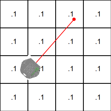
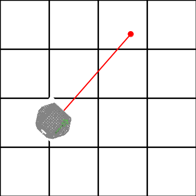
   Assume that the initial distribution is uniform, the robot is not moving, and that sensor readings are independent given the robot's position. (I.e. one incorrect sensor reading does not increase the probability of seeing the same incorrect sensor reading in the future.)

2. Consider a robot mapping it's environment using a laser range finder. The following figure illustrates the initial occupancy grid as well as the first sensor reading. The red line indicates the path taken by the laser, and the red dot is based on the the reported range value. In this case there was an obstacle detected in map cell (0,2).

   

   We will assume that the robot's position is known, and that we have the following sensor model for our laser:

   P( z_t = hit | m_x,y ) = .8
   P( z_t = free | m_x,y ) = .2
   P( z_t = hit | m_x,y ) = .1
   P( z_t = free | m_x,y ) = .9
   

   Where P(m_x,y) expresses the probability that grid cell (x,y) is occupied and P(m_x,y) is the the probability that the cell is free. The expression z_t = hit indicates that the cell in question contains end-point of the laser, and the expression z_t = free indicates that the laser passed through the cell without a collision. (We don't have any new evidence about cells that the laser didn't pass through, so their occupancy probabilities will not be updated.)

   • Apply Baye's rule to update the robot's occupancy grid. In other words, calculate P(m_x,y | z_t) for each cell.

     

   • Perform an additional update assuming that the robot receives exactly the same sensor reading on the next time step.

     
3. Repeat the previous exercise using the occupancy grid mapping algorithm described in Table 1 of Learning Occupancy Grid Maps with Forward Sensor Models¹. This algorithm requires an inverse sensor model of the form P( m_x,y | z_t). Use the following model for this question:
   
   P( m_x,y | z_t = hit) = .9
   P( m_x,y | z_t = free) = .2
   

   • Initial log-odds values given an initial occupancy probability of .1:

     

   • Log-odds values after one update:

     

   • Log-odds values after the second update:

     

---

1. There is a typo in "Recovery of Occupancy Probabilities" section of the algorithm. The equation p(m_x,y, | z₁, ... , z_T) = 1 - 1 / e^l_x,y should be p(m_x,y, | z₁, ... , z_T) = 1 - 1 /(1 + e^l_x,y)