Reliability

Reliability
An Introduction

Prof. David Bernstein
James Madison University

Computer Science Department

bernstdh@jmu.edu

Definitions

Rugged:
- Reliable - Low probability of failure under normal operating conditions
- Robust - Able to operate under a wide variety of condtions
- Safe - Able to minmize the damage resulting from failure
(Probabilistic) Reliability:
- The probability that a system will perform its required functions (without failure) in a particular environment for a particular amount of time

Different Kinds of Systems

Non-Repairable:
- The system can't be repaired after it fails
- Our concern is with measures like the probability of a failure and the remaining life
Repairable:
- The system can be repaired after it fails
- Our concern is with measures like the probability that it won't fail, the time between failures, and the availability

Failure Patterns

Increasing Failure Rate:
- Usually a result of deterioration
Decreasing Failure Rate:
- Usually a result of "hardening" or "burn-in"
- Usually temporary
Constant Failure Rate:
- Usually a result of "stress"/"overload" (i.e., beyond normal operating conditions)

Differences between Hardware and Software

Hardware	Software
Components can "burn in" and "wear out"	Components do not "burn in" or "wear out"
Variation across "copies"	No variation across "copies"

Mathematical Preliminaries

The Setting:
- A system that we are considering over a time interval \([0,t]\)
Our Concern:
- \(R\) - the reliability of the system over the interval

Some Notation

Component Performance:
- \(X_i\) is 1 if the component performs adequately over the interval and 0 otherwise
System Performance:
- \(\phi(X_1, X_2, \ldots, X_n)\) is 1 if the system performs adequately over the interval and 0 otherwise

Archetypical Systems

Series Systems:
- The system fails if any of its components fails
- \(\phi(X_1, X_2, \ldots, X_n) = \min\{X_1, X_2, \ldots, X_n\}\)
Parallel Systems:
- The system fails if all of its components fails
- \(\phi(X_1, X_2, \ldots, X_n) = \max\{X_1, X_2, \ldots, X_n\}\)

Reliability of Archetypical Systems

Series System:
- \(R = P\{\min(X_1, X_2, \ldots, X_n) = 1\} = P\{X_1=1, X_2=1, \ldots, X_n=1\}\)
- If the components are independent, \(R = P\{X_1=1\} \cdot P\{X_2=1\} \cdots \cdot P\{X_n=1\}\)
Parallel Systems:
- \(R = P\{ \max\{X_1, X_2, \ldots, X_n\} = 1\} = 1 - P\{X_1=0, X_2=0, \ldots, X_n=0\}\)
- If the components are independent, \(R = 1 - (1-P\{X_1=1\}) \cdot (1-P\{X_2=1\}) \cdots \cdot (1-P\{X_n=1\})\)

Examples Involving Archetypical Systems

Series System:
- Suppose we have two networks that are connected by a single path consisting of four routers
- Suppose further that the routers have probabilities of working of 0.9, 0.8, 0.9, and 0.7.
- The reliability of the path working is \(R = 0.9 \cdot 0.8 \cdot 0.9 \cdot 0.7 = 0.45\)
Parallel System:
- Suppose we have an electronic commerce site that has four servers all providing the same services
- Suppose further that the servers have probabilities of working of 0.9, 0.8, 0.9, and 0.7.
- The reliability of the site working is \(R = 1 - (1-0.9) \cdot (1-0.8) \cdot (1-0.9) \cdot (1-0.7) = 1 - (.1)(.2)(.1)(.3) = 1 - 0.0006 = 0.9994\)

\(k\) Out of \(n\) Systems

Defined:
- The system operates adequately if any \(k\) out of \(n\) components operate adequately
An Implication:
- \(\phi(X_1,X_2,\ldots,X_n) = \left\{ \begin{array}{l l} \text{1 if }\sum_{i=1}^{n}X_i \geq k \\ \text{0 if }\sum_{i=1}^{n}X_i \lt k \end{array} \right. \)

Reliability of \(k\) Out of \(n\) Systems

In General:
- Finding the reliability for such systems is very complicated
An Important Special Case:
- All of the components are independent and have the same probability of failure, \(p\). In this case, \(\sum_{i=1}^{k}X_i\) has a binomial distribution so:
- \(R = \sum_{i=k}^{n} \left( \begin{array}{c}n \\ i\end{array} \right) p^i (1 - p)^{n-i} \)
Recall:
- \(\left( \begin{array}{c}n \\ i\end{array} \right) = \frac{n!}{i!(n-i)!}\)

An Example of a \(k\) Out of \(n\) System

The System:
- Suppose we have a disk array that can continue to work adequately if any 4 out of 8 disks is working adequately
- Suppose further that each disk has a probability of 0.95 of working adequately
The Reliability:
- \(R = \sum_{i=4}^{8} \left( \begin{array}{c}8 \\ i\end{array} \right) (0.95)^i (0.05)^{8-i} = 0.9999 \)

Reliability of Networks

More General Systems:
- We would like to consider the reliability of systems that can be represented as graphs
An Example:
- Traffic can move from A to D if 1 and 4 are operating, or if 2 and 5 are operating, or if 1 and 3 and 5 are operating

Reliability of Networks (cont.)

An Observation:
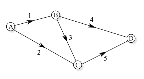
- Since there are 5 edges and each can be working or not, there are \(2^5 = 32\) realizations to consider
The System Reliability:
- Determine the probability of each realization
- Add the probabilities of the realizations that contain a path

Reliability of Networks - A Better Way

Minimal Paths:
- A minimal set of components that by functioning ensure the function of the system
Minimal Cuts:
- A minimal set of components that by failing ensure the failure of the system
Finding the Reliability using Minmal Paths:
- The system will operate if all of the components in at least one of the minimal paths operate
Finding the Reliability using Minmal Cuts:
- The system will fail if and only if all the components in at least one of the minmal cuts fail

Dynamic Software Reliability Models

Objective:
- Predict the failure rate as a function of the number of defects/faults in the system
- Determine the amount of testing time (and subsequent debugging) required to reduce the failure rate to a given threshold
The Process being Modeled:
- The software initially has an unknown number of defects/faults
- It is tested for some amount of time during which failures occur
- When a failure occurs the defect/fault is fixed (which is assumed to require no time for simplicity) and no new defects/faults are introduced

Dynamic Software Reliability Models (cont.)

Notation:
- \(N(t)\) denotes the number of defects/faults at time \(t\)
- \(\lambda(t)\) denotes the failure rate at time \(t\)
- \(c\) denotes a constant
- \(M(t) = N(0) - N(t)\) denotes the number of defects/faults found (and corrected) in the interval \([0, t]\)
An Important Caveat:
- The accuracy of these models is not known

The Jelinski-Moranda Model

Assumptions:
- The failure rate is described by a Poisson process that varies with time, specifically, \(\lambda(t) = c N(t)\)
- The testing time between failures is exponentially distributed
The Model:
- \(R(t) = e^{-\lambda(0) t} = e^{-cN(0) t}\)
- Given a failure at time \(\tau\), the probability that the interval \([\tau, \tau+t]\) will be failure free is \(R(t|\tau) = e^{-cN(\tau) t}\)
Criticism:
- It assumes "all faults are created equal" (i.e., all faults contribute equally to the failure rate)

The Jelinski-Moranda Model (cont.)

An Example:
- \(N(0) = 40\)
- \(c = 0.025\)
What We Want to Know:
- The reliability (i.e., the probability that the system will not have a failure) in the first day of testing
- The reliability (i.e., the probability that the system will not have a failure) in the first three days of testing
Applying the Model:
- \(R(1) = e^{-cN(0) \cdot 1} = e^{-0.025 \cdot 40 \cdot 1} = 0.368\)
- \(R(3) = e^{-cN(0) \cdot 3} = e^{-0.025 \cdot 40 \cdot 3} = 0.050\)

The Musa-Okumoto Model

Assumptions:
- \(N(0) = \infty\)
- \(\lambda(0)\) is known and finite
- It is exponentially more difficult to find/cause failures over time, specifically \(\lambda(t) = \lambda(0) e^{-c E[M(t)]}\)
Some Math (You Don't Need to Know):
- The Differential Equation:
- \(\frac{dE[M(t)]}{dt} = \lambda(0) e^{-c E[M(t)]}\)
- The Solution:
- \(E[M(t)] = \frac{\ln(\lambda(0)ct + 1)}{c}\)
- \(\lambda(t) = \frac{\lambda(0)}{\lambda(0)ct + 1}\)
- So:
- \(R(t) = e^{-\int_0^t \lambda(x)dx} = e^{-E[M(t)]}\)
- \(R(t|\tau) = e^{-\int_{\tau}^{\tau+t} \lambda(x)dx} = e^{-E[M(\tau+t)]+E[M(\tau)]}\)
The Result:
- \(R(t) = (1 + \lambda(0) c t)^{-\frac{1}{c}}\)
- \(R(t|\tau) = \left( 1 + \frac{\lambda(0)ct}{1+\lambda(0)c\tau} \right)^{-\frac{1}{c}}\)

The Musa-Okumoto Model (cont.)

An Example:
- \(\lambda(0) = 1\)
- \(c = 0.025\)
What We Want to Know:
- The reliability (i.e., the probability that the system will not have a failure) in the first day of testing
- The reliability (i.e., the probability that the system will not have a failure) in the first three days of testing
Applying the Model:
- \(R(1) = (1 + \lambda(0) c \cdot 1)^{-\frac{1}{c}} = (1 + 1 \cdot 0.025 \cdot 1)^{-\frac{1}{0.025}} = 0.372\)
- \(R(3) = (1 + \lambda(0) c \cdot 3)^{-\frac{1}{c}} = (1 + 1 \cdot 0.025 \cdot 3)^{-\frac{1}{0.025}} = 0.055\)

There's Always More to Learn