Queueing Theory

Queueing Theory
An Introduction

Computer Science Department

bernstdh@jmu.edu

Motivation

A Personal Experience:
- I went to the store at 5:30
- There was an enormous line at each cashier
What Caused the Lines?
- 200 people left work at 5:00 and went to the store
- There were 5 cashiers working
- Each cashier can check-out 50 people per hour
- At 5:30, only 125 people had checked out

Motivation (cont.)

Motivation (cont.)

Motivation (cont.)

Motivation (cont.)

A Conceptual Model

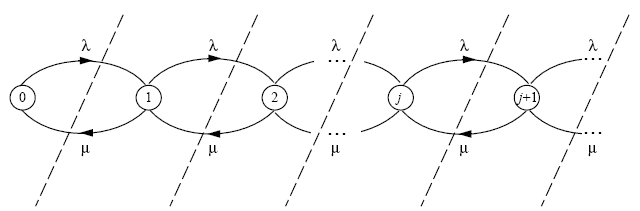
$\lambda$ denotes the arrival rate
$\mu$ denotes the service rate

Going Further

: Modeling State Transitions in Queues

Visualizing Transitions:
A Steady State:
- $\lambda \cdot P\{Q(t) = j \} = \mu \cdot P\{Q(t) = j+1 \}$ for all $j$

Going Further

: Modeling Steady States in Queues

Simplifying the Notation:
- We can ignore $t$ since we are in a steady state
- So, let $P_j$ denote the probability that there are $j$ people in the system when it has "settled down"
Stability Revisited:
- $P_{j+1} = \frac{\lambda}{\mu} P_j$ for all $j$

Going Further

: Modeling Steady States in Queues

Interarrival times are identically and independently distributed
Interarrival times are exponentially distributed (i.e., have the memoryless property)

Service times are identically and independently distributed
Service times are exponentially distributed (i.e., have the memoryless property)

Going Further

: Modeling Steady States in Queues (cont.)

Some Particular Cases:
- $P_{1} = \frac{\lambda}{\mu} P_0$
- $P_{2} = \frac{\lambda}{\mu} ( \frac{\lambda}{\mu} P_0 ) = ( \frac{\lambda}{\mu} )^2 P_0$
- $P_{n} = ( \frac{\lambda}{\mu} )^n P_0$
Letting \rho = \lambda / \mu:
- $P_{n} = \rho^n P_0$

Going Further

: Modeling Steady States in Queues (cont.)

What About P_0?
- We know the probabilities must sum to 1
- So, $P_0 + P_1 + P_2 + P_3 + \cdots = 1$
Solving:
- $P_0 + \rho P_0 + \rho^2 P_0 + \rho^3 P_0 + \cdots = 1$
- $\Rightarrow P_0 (1 + \rho + \rho^2 + \rho^3 + \cdots) = 1$
- $\Rightarrow P_0 = \frac{1}{(1 + \rho + \rho^2 + \rho^3 + \cdots)}$
- We know the infinite geometric series $(1 + \rho + \rho^2 + \rho^3 + \cdots)$ equals $1/(1-\rho)$ since $\rho \lt 1$
- Hence, in such cases (i.e., when the arrival rate is less than the service rate) $P_0 = (1 - \rho)$ and $P_n = (1 - \rho) \cdot \rho^n$

Going Further

: Modeling Steady States in Queues (cont.)

Expected Size of the System:
- $0 \cdot P_0 + 1 \cdot P_1 + 2 \cdot P_2 + \cdots = \rho / (1 - \rho) = \lambda / (\mu - \lambda)$
Expected Time in the System:
- The expected number of people in the system must equal the arrival rate times the expected time in the system
- So, the expected time is the expected size divided by the arrival rate
- So, the expected time is $1 / (\mu - \lambda)$

Summary of the Important Results

Probability of n People in the Queue:
- $P_0 = (1 - \lambda/\mu)$
- $P_n = (1 - \lambda/\mu) \cdot (\lambda/\mu)^n$
Expected Size of the System:
- $\lambda / (\mu - \lambda)$
Expected Time in the System:
- $1 / (\mu - \lambda)$

An Example

The Data:
- Arrival rate is 30 per hour
- Service rate is 40 per hour
The Expected Steady State Values:
- Size: 30/(40-30) = 3 people
- Time: 1/(40-30) = 1/10 hours

Designing Queueing Systems

Service Mechanism:
- Number of servers
- Number of waiting lines (one common line, one line for each server)
- Service rate (if it can be controlled)
Queueing Discipline:
- First-come-first-served
- Last-come-first-served
- Priority (or preemptive) service
- Shortest remaining processing time

There's Always More to Learn