|
Equilibrium Route Choice
An Introduction |
|
Prof. David Bernstein
|
| Computer Science Department |
| bernstdh@jmu.edu |

|
Equilibrium Route Choice
An Introduction |
|
Prof. David Bernstein
|
| Computer Science Department |
| bernstdh@jmu.edu |

A Failed Attempt
Equilibrium
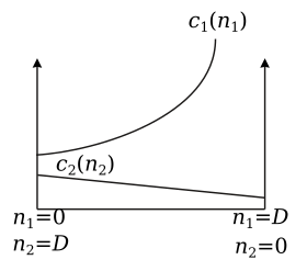
Other Interesting Examples
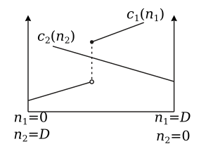
Other Interesting Examples (cont.)
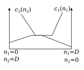
Other Interesting Examples (cont.)
Other Interesting Examples (cont.)
Other Interesting Examples (cont.)