Curves in 2 or 3 Dimensions (Plane or Space Curves)

Curves in 2 or 3 Dimensions (Plane or Space Curves)
An Introduction

Computer Science Department

bernstdh@jmu.edu

Review of our Discussion of Lines in 2D

Explict Form [y=f(x)]:
- $p_2(p_1) = m p_1 + b$
Implict Form [f(x,y)=0]:
- $\bs{n} \cdot \bs{p} + b = 0$
Parametric Form [x=f(\lambda), y=g(\lambda)]:
- $\bs{p}(\lambda) = \lambda \bs{r} + (1 - \lambda) \bs{s}$

What About Curves?

Explicit Form:
- Explict representations often don't exist (e.g., a circle around the origin with radius $r$ requires two functions, $y = \sqrt{r^2 - x^2}$ and $y = -\sqrt{r^2 - x^2}$ , and they only hold when $0 \leq |x| \leq r$ )
Implicit Form:
- We can use implicit representations (e.g., a circle around the origin with radius $r$ can be represented as $x^2 + y^2 - r^2 = 0$ )
- But, we must use a scanning algorithm (i.e., check each point to see if it is on the curve)
- In addition, curves in 3D are difficult to represent in implicit form (it is possible to use the intersection of surfaces but it is difficult)

Parametric Polynomial Curves

A Curve of Degree n:
- $\bs{p}(\lambda) = \sum_{k=0}^{n} \bs{c_k} \lambda^k$
Be Careful:
- $\bs{c_k}$ has as many components as $\bs{p}$ . That is, $\bs{c_k} = [ c_{k1} \;\; c_{k2} \;\; c_{k3} ]^T$

Parametric Cubic Polynomial Curves

The Representation:
- $\bs{p}(\lambda) = \bs{c_0} + \bs{c_1} \lambda + \bs{c_2} \lambda^2 + \bs{c_3} \lambda^3$
A Cubic in Matrix Form:
- $\bs{C} = \left[ \begin{array}{r r r} c_{01} && c_{11} && c_{21} && c_{31} \\ c_{02} && c_{12} && c_{22} && c_{32} \\ c_{03} && c_{13} && c_{23} && c_{33} \\ \end{array}\right]$
- $\bs{\lambda} = \left[ \begin{array}{r}1 \\ \lambda \\ \lambda^2 \\ \lambda^3 \end{array}\right]$
- $\bs{p} = \bs{C} \bs{\lambda}$

Parametric Cubic Polynomial Curves (cont.)

The Interpolating Polynomial:
- Given four points (i.e., 12 independent variables), we can find the coefficients, $\bs{C}$ , of a cubic polynomial curve that pass through them
Other Related Approaches:
- Hermite curves
- Parabolic blending

Bézier Curves

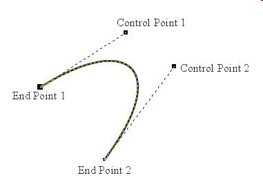
The Idea:
- Use four points, $\bs{q}_0, \bs{q}_1, \bs{q}_2, \bs{q}_3,$ , but don't have the curve pass through all of them
- Use two, $\bs{q}_0, \bs{q}_3,$ , as the end points and two, $\bs{q}_1, \bs{q}_2$ , to approximate the tangents at the end points
A Visualization:

Bézier Curves (cont.)

Recall:
- $\bs{p}(\lambda) = \bs{c_0} + \bs{c_1} \lambda + \bs{c_2} \lambda^2 + \bs{c_3} \lambda^3$
The Obvious Conditions:
- $\bs{p}(0) = \bs{q}_0 \Rightarrow \bs{c_0} = \bs{q}_0$
- $\bs{p}(1) = \bs{q}_3 \Rightarrow \bs{c_0} + \bs{c_1} + \bs{c_2} + \bs{c_3} = \bs{q}_3$
Linear Approximations of the Tangents:
- Assuming that the points are evenly spaced, they correspond to $\lambda=0$ , $\lambda=1/3$ , $\lambda=2/3$ , and $\lambda=1$ . So:
- An approximation of the tangent at $\lambda=0$ is given by $\frac{\bs{q}_1 - \bs{q}_0}{1/3}$ (or, equivalently, $3(\bs{q}_1 - \bs{q}_0)$ )
- An approximation of the tangent at $\lambda=1$ is given by $\frac{\bs{q}_3 - \bs{q}_2}{1/3}$ (or, equivalently, $3(\bs{q}_3 - \bs{q}_2)$ )
The Derivative:
- $\frac{d \bs{p}(\lambda)}{d \lambda} = \bs{c_1} + 2 \bs{c_2} \lambda + 3 \bs{c_3} \lambda^2$
The Tangency Conditions:
- $\left.\frac{d \bs{p}(\lambda)}{d \lambda}\right|_{\lambda = 0} = 3 \bs{q}_1 - 3 \bs{q}_0 \Rightarrow \bs{c_1} = 3 \bs{q}_1 - 3 \bs{q}_0$
- $\left.\frac{d \bs{p}(\lambda)}{d \lambda}\right|_{\lambda = 1} = 3 \bs{q}_3 - 3 \bs{q}_2 \Rightarrow \bs{c_1} + 2 \bs{c_2} + 3 \bs{c_3} = 3 \bs{q}_3 - 3 \bs{q}_2$

Bézier Curves (cont.)

On Way to Proceed:
- Solve this system of equations
Another Way to Proceed:
- Recognize that this is an application of Bernstein polynomials
- $B_{i,n}(\lambda) = \left( \begin{array}{c c} n \\ i \end{array} \right) (1 - \lambda)^{n-i} \lambda^i$

Bézier Curves (cont.)

Bernstein Representation:
- An $n$ th-order Bézier curve can be written in terms of $n+1$ points, $\bs{q}_0, \ldots, \bs{q}_n$ , as follows
- $\bs{p}(\lambda) = \sum_{i=0}^{n} B_{i,n}(\lambda) \bs{q}_i$
Cubic Bézier Curves Revisited:
- $\bs{p}(\lambda) = B_{0,3}(\lambda) \bs{q}_0 + B_{1,3}(\lambda) \bs{q}_1 + B_{2,3}(\lambda) \bs{q}_2 + B_{3,3}(\lambda) \bs{q}_3$
- where
- $B_{0,3}(\lambda) = -\lambda^3 + 3\lambda^2 - 3\lambda + 1$
- $B_{1,3}(\lambda) = 3\lambda^3 - 6\lambda^2 + 3\lambda$
- $B_{2,3}(\lambda) = -3\lambda^3 + 3\lambda^2$
- $B_{3,3}(\lambda) = \lambda^3$

Cubic Bézier Curves

Expanding:
- $\bs{p}(\lambda) = ( -\lambda^3 + 3\lambda^2 - 3\lambda + 1) \bs{q}_0 + ( 3\lambda^3 - 6\lambda^2 + 3\lambda) \bs{q}_1 + (-3\lambda^3 + 3\lambda^2) \bs{q}_2 + ( \lambda^3) \bs{q}_3$
Collecting Terms:
- $\bs{p}(\lambda) = (- \bs{q}_0 + 3 \bs{q}_1 - 3 \bs{q}_2 + \bs{q}_3) \lambda^3 + (3 \bs{q}_0 - 6 \bs{q}_1 + 3 \bs{q}_2) \lambda^2 + (-3 \bs{q}_0 + 3 \bs{q}_1) \lambda + (\bs{q}_0) 1$
Matrix Notation:
- $\bs{p}(\lambda) = \left[ \begin{array}{l l l l} q_{01} & q_{11} & q_{21} & q_{31} \\ q_{02} & q_{12} & q_{22} & q_{32} \\ q_{03} & q_{13} & q_{23} & q_{33} \\ \end{array} \right] \left[ \begin{array}{r r r r} -1 & 3 & -3 & 1 \\ 3 & -6 & 3 & 0 \\ -3 & 3 & 0 & 0 \\ 1 & 0 & 0 & 0 \\ \end{array} \right] \left[ \begin{array}{l} \lambda^3 \\ \lambda^2 \\ \lambda \\ 1 \\ \end{array} \right]$

Bézier Curves (cont.)

Some Interesting Observations:
- $B_{i,n}(\lambda) \in (0, 1]$
- $\sum_{i=1}^{n} B_{i,n}(\lambda) = 1$
The Implications:
- $\bs{p}(\lambda) = \sum_{i=0}^{n} B_{i,n}(\lambda) \bs{q}_i$ is a convex combination of $\bs{q}_0, \ldots, \bs{q}_n$
- The curve is in the convex hull formed by $\bs{q}_0, \ldots, \bs{q}_n$

There's Always More to Learn